set.seed(2025115)
graded_question <- sample(9,size = 1)
paste("Question",graded_question,"is the graded question for this week")
[1] "Question 7 is the graded question for this week"In this lab, we’ll explore data from the National Election Studies 2024 Pilot Study. You find an outcome of interest and a variable you think predicts interesting variation in that outcome. You’ll figure out what recoding you need to do, do that recoding and describe the data. I’ll do the same, so can some template code to compare your work to.
Everything we’ll do today is something we’ve done before and is also something you’ll likely have to do a version of in your final project. Here’s the plan
Set up your work space
Download and load data from the NES into R
Explore the codebook for the 2024 Pilot Study
Get a high level overview of the data to figure out what recoding needs to be done
Recode the data
Describe the data
Formulate a set of research questions
Estimate models to explore your question
Interpret the results of your model
One of these 9 tasks will be randomly selected as the graded question for the lab.
set.seed(2025115)
graded_question <- sample(9,size = 1)
paste("Question",graded_question,"is the graded question for this week")[1] "Question 7 is the graded question for this week"This week’s lab will give you practice:
Download and loading data from your own computers (Q1,Q2)
Exploring a codebook to find interesting relevant variables (Q3)
Exploring data to understand what needs to be recoded (Q4)
Recoding data in a clear and precise manner (Q5)
across()Describing, summarizing, and exploring data through tables and figures (Q6)
kable() and functions from the kableExtra package to format tablesggarrange()from the `ggpubr pacakgeFormulating research questions based on initial explorations of the data (Q7)
Estimating linear models (Q8)
Interpreting the substantive and statistical significance of these models (Q9)
As with every lab, you should:
author: section of the YAML header.In the code chunk below, please add code to load the package DeclareDesign
# Libraries
library(tidyverse)
library(haven)
library(labelled)
library(kableExtra)
library(ggpubr)
library(DeclareDesign)In R studio set your working directory to the folder where this lab is saved by clicking > Session > Set Working Directory > To Source File Location

After doing so uncomment getwd() Should print out something like
“~/Desktop/pols2580/labs/”
Depending on where your lab is saved
# In the Top Panel of RStudio Click
# Session > Set Working Directory > Source File Location

# Uncomment to Check Where Your File is Saved
# getwd()If getwd() says something like ‘~/Downloads/’ click: “File > Save As” and save this lab in your course folder. Then close the version 09-lab.qmd that was opened from your Downloads folder and open the version of 09-lab.qmd that now exists in your course folder.
Please click here to go to the download page for the National Election Studies 2024 Pilot Study

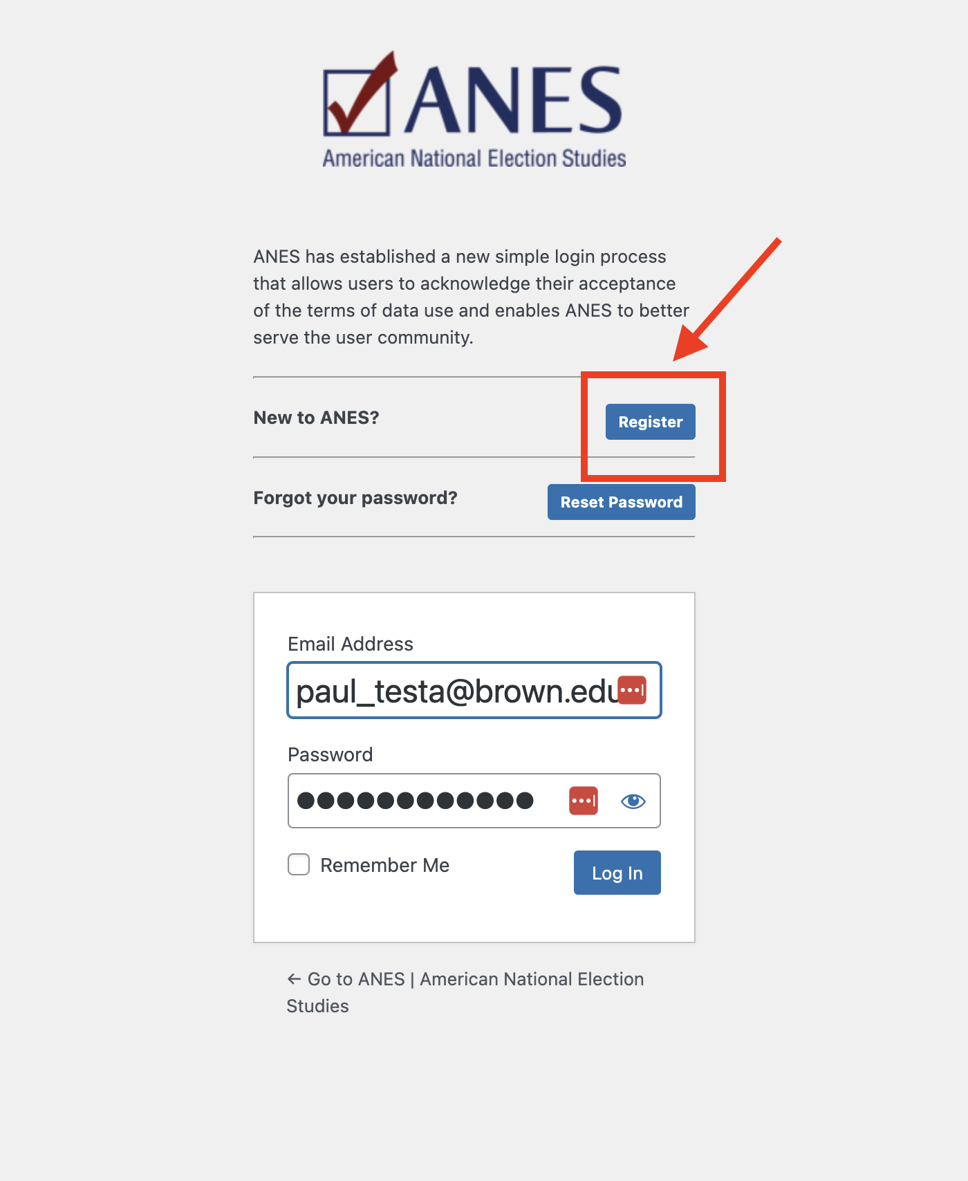
Save Link As... Which should in turn allow you to chose where the file is saved. Save it in the same folder as 09-lab.qmd

anes_pilot_2024_dta_20240319.zip.
anes_pilot_2024_dta_20240319 in your course folder which contains the following files:anes_pilot_2024_dta_20240319.dta the dataanes_pilot_2024_userguidecodebook_20240319.pdf the codebook for the data
## IF .dta file is in subfolder where lab is:
# df <- read_dta("~/anes_pilot_2024_dta_20240319/anes_pilot_2024_20240319.dta")

## IF .dta file is in SAME folder as lab:
# df <- read_dta("anes_pilot_2024_20240319.dta")

## IF nothing works, fear not, you can load the data from the web as a backup
df <- read_dta(url("https://pols2580.paultesta.org/files/data/anes_pilot_2024_20240319.dta"))Please open the file anes_pilot_2024_userguidecodebook_20240319.pdf.
It should be in same folder as the data.
Use Control+F for keywords to quickly navigate through the codebook looking for questions and variables that interest you.
In this and next week’s lab, I’ll be exploring factors that explain variation in the following outcome variables:
A measure
vchoice_rematch “Vote Trump or Biden in 2024”
1 = Donald Trump2 = Joe Biden-7 = No Answer-1 = InapplicableAnd five measures of political participation in the 2020 campaign
mobil_talk “2020 campaign - Talk to others about candidates”
mobil_online “2020 campaign - Participate in online rallies”
mobil_rally “2020 campaign - Attend in person rallies”
mobil_button “2020 campaign - Wear a button or campaign sticker”
mobil_work “2020 campaign - Any other work to support candidates”
1 = Yes2 = No-1 = InapplicablePlease find a variable that describes some outcome of interest to you and fill in the following
outcome_variable_name Question topic
From a quick skim, I’ve selected the following potential predictors, which I will recode below:
age Ageeduc Educationfaminc_new Incomerace Racepid7 7 point party identificationPlease find at least one more predictor which you think might explain variation in your outcome of interest and fill in the following
predictor_variable_name Question topic
For example, perhaps you’re interested in differences by gender, or ideology, or social media use. See if you can find variables that measure these concepts.
You only needed to identify one, but you can choose to explore more if you want. Don’t choose 50, unless you really like recoding data.
In this section, we’ll get practice quickly looking at variables to see what, if anything needs to be recoded.
I had you download the .dta instead of the .csv version of the data, because the .dta includes value labels for the data, which makes it easier to understand what a specific number corresponds to substantively.
Please uncomment and run the code below
# Vote Choice
get_variable_labels(df$vchoice_rematch)
[1] "Vote Trump or Biden in 2024"get_value_labels(df$vchoice_rematch) No Answer inapplicable, legitimate skip
-7 -1
Donald Trump Joe Biden
1 2
8 9 table(df$vchoice_rematch,useNA = "ifany")
 -7  -1   1   2
 23 151 869 866
# Acts of Participation
# All variables start with mobil_ prefix
df %>% select(starts_with("mobil")) %>% names() [1] "mobil_talk" "mobil_online" "mobil_rally"
[4] "mobil_button" "mobil_work" "mobil_talk_skp"
[7] "mobil_online_skp" "mobil_rally_skp" "mobil_button_skp"
[10] "mobil_work_skp" "mobil_talk_pg_timing" "mobil_online_pg_timing"
[13] "mobil_rally_pg_timing" "mobil_button_pg_timing" "mobil_work_pg_timing" # Political Talk
get_variable_labels(df$mobil_talk)[1] "2020 campaign - Talk to others about candidates"get_value_labels(df$mobil_talk) No Answer inapplicable, legitimate skip
-7 -1
Yes No
1 2
8 9 table(df$mobil_talk,useNA = "ifany")
  -7   -1    1    2
   1  150  704 1054
# Save the names all variables related to acts of participation in 2020
the_participation_vars <- df %>% select(starts_with("mobil")) %>% names()
# Only keep the variables that measure participation and not survey timing
the_participation_vars <- the_participation_vars[1:5]From quickly looking at my outcome variables, I know that I will want to:
vchoice_rematch to dv_vote_trump2024 which
vchoice_rematch == 1vchoice_rematch == 2NA if vchoice_rematch < 0mobil_* to variables that start with polpart_* and:
mobil_* == 1mobil_* == 2NA if mobil_* < 0`dv_participation* which is the sum of respondents’ five responses to the recoded polpart_* variablesIn the code chunk below, please repeat this process for the outcome variable you selected in the previous section:
# Get a HLO of your outcome variableYOUR OUTCOME VARIABLE HERE to NAME FOR RECODED VARIABLE
Now I’ll repeat this process for my potential predictor variables.
Please uncomment and run the code below
# Age
get_variable_labels(df$age)
[1] "Profile variable: Age"get_value_labels(df$age)not asked
-9 summary(df$age) Min. 1st Qu. Median Mean 3rd Qu. Max.
-9.00 33.00 51.00 48.43 63.00 94.00 # Education
get_variable_labels(df$educ)[1] "Profile variable: Education"get_value_labels(df$educ) No HS credential High school graduate Some college
1 2 3
2-year degree 4-year degree Post-grad
4 5 6 table(df$educ)
  1   2   3   4   5   6
84 584 381 210 426 224 summary(df$educ) Min. 1st Qu. Median Mean 3rd Qu. Max.
1.000 2.000 3.000 3.514 5.000 6.000 # Income
get_variable_labels(df$faminc_new)[1] "Profile variable: Family income"get_value_labels(df$faminc_new) No Answer inapplicable, legitimate skip
-7 -1
Less than $10,000 $10,000 - $19,999
1 2
$20,000 - $29,999 $30,000 - $39,999
3 4
$40,000 - $49,999 $50,000 - $59,999
5 6
$60,000 - $69,999 $70,000 - $79,999
7 8
$80,000 - $99,999 $100,000 - $119,999
9 10
$120,000 - $149,999 $150,000 - $199,999
11 12
$200,000 - $249,999 $250,000 - $349,999
13 14
$350,000 - $499,999 $500,000 or more
15 16
Prefer not to say
97 998
999 table(df$faminc_new)
 -7   1   2   3   4   5   6   7   8   9  10  11  12  13  14  15  16  97
38 119 126 222 142 141 140 122 149 144 120 109 88 31 20 10 4 184 summary(df$faminc_new) Min. 1st Qu. Median Mean 3rd Qu. Max.
-7.00 3.00 7.00 14.89 10.00 97.00 # Race
get_variable_labels(df$race)[1] "Race"get_value_labels(df$race) No Answer inapplicable, legitimate skip
-7 -1
White Black
1 2
Hispanic Asian
3 4
Native American Two or more races
5 6
Other Middle Eastern
7 8
98 99 summary(df$race) Min. 1st Qu. Median Mean 3rd Qu. Max.
1.000 1.000 1.000 1.751 2.000 8.000 table(df$race,useNA = "ifany")
   1    2    3    4    5    6    7    8
1270  242  239   44   17   69   27    1
# Partisanship
get_variable_labels(df$pid7)[1] "Profile variable: 7 point party identification"get_value_labels(df$pid7) Strong Democrat Not very strong Democrat
1 2
Lean Democrat Independent
3 4
Lean Republican Not very strong Republican
5 6
Strong Republican Not sure
7 8
Don't know
9 summary(df$pid7) Min. 1st Qu. Median Mean 3rd Qu. Max. NA's
1.000 2.000 4.000 4.023 6.000 8.000 58 table(df$pid7)
  1   2   3   4   5   6   7   8
389 228 173 295 172 184 342  68
After taking a quick look at each variable, I know that I’ll want to do the following recoding:
age to age1
-9s to NAeduc no recoding needed
has_college_degree which equals 1 is educ > 4 and 0 otherwisefaminc_new to income
-7 and 97 to NArace to race_5cat
race == 1 ~ "White"race == 2 ~ "Black"race == 3 ~ "Hispanic"race == 4 ~ "Asian"T ~ "Other" (Collapse other racial categories)race to is_* binary indicators:
is_white = 1 if race==1, 0 otherwisepid7 to partyid
pid7 == 8 to 4 (Classify Don't Knows as Independents)pid7 to is_*: binary indicators:
is_dem = 1 if partyid < 4, 0 otherwiseis_rep = 1 if partyid > 4, 0 otherwiseis_ind = 1 if partyid == 4, 0 otherwiseIn the code chunk below, please repeat this process for the additional predictor(s) you selected in the previous section:
# Get a HLO of your outcome variableYOUR OUTCOME VARIABLE HERE to NAME FOR RECODED VARIABLE
Now we’ve got a plan of action for how we need to recode the data.
Please uncomment and run the following code chunk:
df %>%
  # Recode 2024 Vote Choice
  mutate(
    dv_vote_trump2024 = case_when(
      vchoice_rematch == 1 ~ 1,
      vchoice_rematch == 2 ~ 0,
      T ~ NA
    )
  ) %>%
  # Recode Individual Acts of Participation
  mutate(across(all_of(the_participation_vars),
                \(x) case_when(
                  x == 1 ~ 1,
                  x == 2 ~ 0,
                  T ~ NA
                ),
                .names = "polpart_{.col}"
                )

                ) %>%
  # Create Additive Measure of Participation
  mutate(
    dv_participation = rowSums(
      select(.,starts_with("polpart")),
      na.rm = T)

  ) -> df
Please recode your outcome of interest as needed
Remember to save the output of your recode back into the dataframe df
# Recode your outcome of interestIt’s a good habit to compare your recoded variables to their original values, to make sure your code did what you thought it did.
Please uncomment and run the following:
# Check recodes

table(
  recode = df$dv_vote_trump2024,
  original = df$vchoice_rematch,
  useNA = "ifany"
  )
original
recode -7 -1 1 2
0 0 0 0 866
1 0 0 869 0
<NA> 23 151 0 0table(
recode = df$polpart_mobil_button,
original = df$mobil_button,
useNA = "ifany"
) original
recode -1 1 2
0 0 0 1386
1 0 373 0
<NA> 150 0 0table(
total = df$dv_participation,
item = df$polpart_mobil_button,
useNA = "ifany"
) item
total 0 1 <NA>
0 884 0 149
1 364 62 1
2 89 109 0
3 38 71 0
4 11 83 0
5 0 48 0So everything looks in order. I could have probably checked the dv_participation variable against all of its constituent items, but based off comparing it to polpart_mobil_button everything looks in order since: - there are no cases where polpart_mobil_button is 1 but dv_participation is 0 - there are no cases where dv_participation is at it’s max but polpart_mobil_button is 0. - dv_participation has the correct theoretical range from 0 acts to 5 acts.
Now do the same for your outcome variable.
Please check your recoded outcome against its original values
# Check recodesAgain, I’ve provide some demonstration code to recode the predictors listed above.
Please uncomment and run the following
df %>%
  mutate(
    # Age
    age = ifelse(age < 0, NA, age),
    # Education
    education = educ,
    educ_f = to_factor(educ), #Convert to Factor for Plotting
    is_college_grad = ifelse(educ > 4,1,0),
    # Income
    income = case_when(
      faminc_new < 0 ~ NA,
      faminc_new > 0 & faminc_new >16 ~ NA,
      T ~ faminc_new
    ),
    # Race
    race_5cat = case_when(
      race < 5 ~ to_factor(race),
      T ~ "Other"
    ) %>% factor(., levels = c("White","Black","Hispanic","Asian","Other")),
    is_white = ifelse(race == 1, 1, 0),
    is_black = ifelse(race == 2, 1, 0),
    is_hispanic = ifelse(race == 3, 1, 0),
    is_asian = ifelse(race == 4, 1, 0),
    is_other = ifelse(race == 5, 1, 0),
    # Partisanship
    partyid = case_when(
      pid7 == 8 ~ 4,
      T ~ pid7
    ),
    is_dem = ifelse(partyid  < 4, 1, 0),
    is_rep = ifelse(partyid  > 4, 1, 0),
    is_ind = ifelse(partyid  == 4, 1, 0),
  ) -> df
Please recode your additional predictor(s) as needed
# Recode your additional predictor(s)It’s a good habit to check your all your recoding – particularly if you’re doing something like summing over multiple columns – but for this lab, we’ll live dangerously.
Now let’s get some practice summarizing our data, presenting these summaries as tables and figures, and interpreting our results
Please uncomment and run the code below which demonstrates how to produce a nicely formatted table of summary statistics
# Vector of numeric variables to summarize
the_vars <- c(
  "dv_vote_trump2024",
  "dv_participation",
  "age","education","income",
  "is_white","is_black","is_hispanic","is_asian","is_other",
  "partyid","is_dem","is_rep","is_ind"
)

# Vector of nicely formatted labels for variables
the_labels <- c(
  "Vote for Trump in '24",
  "Acts of Participation in `20",
  "Age","Education", "Income",
  "White", "Black","Hispanic","Asian","Other",
  "Party ID", "Democrat","Republican","Independent"
)

df_summary <- df %>%
  select(all_of(the_vars)) %>%
  rename_with(~the_labels) %>%
  pivot_longer(
    cols = everything(),
    names_to = "Variable"
  ) %>%
  mutate(
    Variable = factor(Variable, levels = the_labels)
  ) %>%
  group_by(Variable) %>%
  summarise(
    Min = min(value,na.rm = T),
    p25 = quantile(value, prob = .25,na.rm = T),
    Median = quantile(value, prob = .5,na.rm = T),
    Mean = mean(value, na.rm = T),
    p75 = quantile(value, prob = .75,na.rm = T),
    Max = max(value,na.rm = T),
    `N missing` = sum(is.na(value))
  )

# Look at results
df_summary
# A tibble: 14 × 8
Variable Min p25 Median Mean p75 Max `N missing`
<fct> <dbl+lb> <dbl> <dbl> <dbl> <dbl> <dbl+lb> <int>
1 Vote for Trump in '… 0 0 1 5.01e-1 1 1 [No … 174
2 Acts of Participati… 0 0 0 9.25e-1 1 5 [4-y… 0
3 Age 18 33 51 4.94e+1 63.8 94 31
4 Education 1 [No … 2 3 3.51e+0 5 6 [Pos… 0
5 Income 1 [No … 3 6 6.43e+0 9 16 [$50… 222
6 White 0 0 1 6.65e-1 1 1 [No … 0
7 Black 0 0 0 1.27e-1 0 1 [No … 0
8 Hispanic 0 0 0 1.25e-1 0 1 [No … 0
9 Asian 0 0 0 2.30e-2 0 1 [No … 0
10 Other 0 0 0 8.91e-3 0 1 [No … 0
11 Party ID 1 [No … 2 4 3.88e+0 6 7 [$60… 58
12 Democrat 0 0 0 4.27e-1 1 1 [No … 58
13 Republican 0 0 0 3.77e-1 1 1 [No … 58
14 Independent 0 0 0 1.96e-1 0 1 [No … 58We can then format df_summary as table using knitr() and styling options from the kableExtra package:
kable(df_summary,
      digits = 2) %>%
  kable_styling() %>%
  pack_rows("Outcomes", start_row = 1, end_row = 2) %>%
  pack_rows("Demographic Predictors", 3, 10) %>%
pack_rows("Political Predictors", 11, 14)| Variable | Min | p25 | Median | Mean | p75 | Max | N missing |
|---|---|---|---|---|---|---|---|
| Outcomes | |||||||
| Vote for Trump in '24 | 0 | 0 | 1 | 0.50 | 1.00 | 1 | 174 |
| Acts of Participation in `20 | 0 | 0 | 0 | 0.93 | 1.00 | 5 | 0 |
| Demographic Predictors | |||||||
| Age | 18 | 33 | 51 | 49.37 | 63.75 | 94 | 31 |
| Education | 1 | 2 | 3 | 3.51 | 5.00 | 6 | 0 |
| Income | 1 | 3 | 6 | 6.43 | 9.00 | 16 | 222 |
| White | 0 | 0 | 1 | 0.67 | 1.00 | 1 | 0 |
| Black | 0 | 0 | 0 | 0.13 | 0.00 | 1 | 0 |
| Hispanic | 0 | 0 | 0 | 0.13 | 0.00 | 1 | 0 |
| Asian | 0 | 0 | 0 | 0.02 | 0.00 | 1 | 0 |
| Other | 0 | 0 | 0 | 0.01 | 0.00 | 1 | 0 |
| Political Predictors | |||||||
| Party ID | 1 | 2 | 4 | 3.88 | 6.00 | 7 | 58 |
| Democrat | 0 | 0 | 0 | 0.43 | 1.00 | 1 | 58 |
| Republican | 0 | 0 | 0 | 0.38 | 1.00 | 1 | 58 |
| Independent | 0 | 0 | 0 | 0.20 | 0.00 | 1 | 58 |
Using the two previous code chunks as a template, update the code so that the table includes your chosen outcome and predictors.
# Copy, paste, and update code from datasummary_me to include your variablesPlease write a few sentences that provide a substantive interpretation of your table of descriptive statistics
Your reader should come away with an understanding of the characteristics of the respondents to this sample.
The National Election Study’s 2024 Pilot Study contains responses from 1909 individuals2. The typical respondent in the data was just under 50 years old, with some college, with an income in the range of $50k-$59k. Approximately two-thirds of the sample identified as white, with 13 percent of respondents identifying as Black, 13 percent as Hispanic, 2 percent as Asian. Forty-three percent of respondents identified as Democrats, 38 percent as Republicans, and 20 percent as Independents. The respondents were evenly split in who they would vote for 2024, with 50 percent saying they would Vote for Donald Trump, and 50 percent saying Joe Biden. In the 2020 campaign, the average respondent reported engaging in about 1 act of political participation.
Note, that technically, 024 Pilot Study contains three types of respondents described by sample_type:
So, technically speaking3, if we wanted to draw inferences about the proportion of American’s planning to to vote for Trump or Biden in 2024, we should only look at the 1,500 respondents in the weighted sample, and we should calculate that proportion using the sampling weights provided by weights.
Survey weights are complicated things, but the basically idea is that each observation is the sample is representative of observations in the population. Some types of observations will be over-represented in our sample – these are given smaller weights – while others are under-represented – these are given greater weights.
Quick look at the highest and lowest survey weights seems to suggest to me that weighting procedure is giving more weight to respondents with lower levels of education, and income, and less weight to higher incomes and education levels.
df %>% filter(
 weight > quantile(weight, .99, na.rm=T)
 ) %>%
  select(weight, gender, age, race_5cat, education, income, partyid)
# A tibble: 15 × 7
weight gender age race_5cat education income partyid
<dbl> <dbl+lbl> <dbl> <fct> <dbl+lbl> <dbl+lbl> <dbl+lb>
1 7.00 1 [Male] 23 Hispanic 3 [Some college] 4 [$30,… 3 [Lea…
2 3.33 1 [Male] 31 Other 2 [High school graduate] NA 2 [Not…
3 2.96 2 [Female] 33 Hispanic 1 [No HS credential] NA 4 [Ind…
4 3.36 1 [Male] 68 Black 3 [Some college] NA 4 [Ind…
5 2.94 1 [Male] 67 Hispanic 1 [No HS credential] 2 [$10,… 2 [Not…
6 4.13 1 [Male] 22 Hispanic 3 [Some college] 11 [$120… 4 [Ind…
7 3.64 2 [Female] 58 Black 5 [4-year degree] 6 [$50,… NA
8 3.30 1 [Male] 43 Hispanic 5 [4-year degree] 7 [$60,… 4 [Ind…
9 3.51 1 [Male] 69 White 2 [High school graduate] 4 [$30,… 7 [Str…
10 3.32 1 [Male] 74 White 2 [High school graduate] 6 [$50,… 3 [Lea…
11 3.32 1 [Male] 69 White 2 [High school graduate] 3 [$20,… 4 [Ind…
12 3.51 1 [Male] 75 White 2 [High school graduate] 2 [$10,… 7 [Str…
13 2.93 1 [Male] 41 Black 4 [2-year degree] 4 [$30,… 2 [Not…
14 4.20 2 [Female] 63 Black 6 [Post-grad] 3 [$20,… 6 [Not…
15 3.32 1 [Male] 67 White 2 [High school graduate] 5 [$40,… 3 [Lea…df %>% filter(
weight < quantile(weight, .01, na.rm=T)
) %>%
select(weight, gender, age, race_5cat, education, income, partyid)# A tibble: 12 × 7
weight gender age race_5cat education income partyid
<dbl> <dbl+lbl> <dbl> <fct> <dbl+lbl> <dbl+lbl> <dbl+l>
1 0.314 1 [Male] 77 Black 6 [Post-grad] 10 [$100,… 1 [Str…
2 0.409 2 [Female] 29 Black 6 [Post-grad] 14 [$250,… 1 [Str…
3 0.382 1 [Male] 23 Hispanic 5 [4-year degree] 10 [$100,… 5 [Lea…
4 0.439 2 [Female] 26 Asian 5 [4-year degree] 12 [$150,… 2 [Not…
5 0.421 2 [Female] 57 Hispanic 6 [Post-grad] 6 [$50,0… 5 [Lea…
6 0.415 2 [Female] 52 Hispanic 6 [Post-grad] 6 [$50,0… 3 [Lea…
7 0.455 1 [Male] 72 Other 6 [Post-grad] 7 [$60,0… 7 [Str…
8 0.405 1 [Male] 32 Hispanic 5 [4-year degree] 11 [$120,… 4 [Ind…
9 0.362 2 [Female] 33 Black 5 [4-year degree] 1 [Less … 1 [Str…
10 0.411 1 [Male] 42 Black 2 [High school graduate] 4 [$30,0… 4 [Ind…
11 0.362 2 [Female] 33 Black 5 [4-year degree] 1 [Less … 1 [Str…
12 0.346 1 [Male] 71 Black 6 [Post-grad] 2 [$10,0… 1 [Str…Sampling weights are a can worms we won’t deal with in this class. Check out these resources on the survey and srvyr packages for how to incorporate survey weights into your analysis. In the code below we see that distributions of race and ethnicity are pretty similar in the weighted and full samples, but using survey weights seems to suggest that Biden’s support as actually higher than Trumps, although the confidence intervals (Next week!) for both overlap 0.5 suggesting the race is essentially tied.
# install.packages("survey")
# install.packages("srvyr")
library(survey)
library(srvyr)

# Format as survey_design object
df_s <- as_survey_design(df %>% filter(sample_type == 1),weight = weight)

# Calculate weighted totals and proportions
df_s %>%
  group_by(race) %>%
  summarise(
    total = survey_total(),
    proption = survey_mean()
  )
# A tibble: 7 × 5
race total total_se proption proption_se
<dbl+lbl> <dbl> <dbl> <dbl> <dbl>
1 1 [White] 1005. 21.6 0.670 0.0139
2 2 [Black] 193. 15.7 0.129 0.0102
3 3 [Hispanic] 189. 15.9 0.126 0.0102
4 4 [Asian] 35.6 6.36 0.0237 0.00423
5 5 [Native American] 11.8 3.26 0.00789 0.00218
6 6 [Two or more races] 46.8 7.52 0.0312 0.00499
7 7 [Other] 17.8 5.53 0.0119 0.00367# Compare to unweighted estimates
df %>%
group_by(race) %>%
summarise(
total = n()
) %>%
mutate(
propotion = total/sum(total)
)# A tibble: 8 × 3
race total propotion
<dbl+lbl> <int> <dbl>
1 1 [White] 1270 0.665
2 2 [Black] 242 0.127
3 3 [Hispanic] 239 0.125
4 4 [Asian] 44 0.0230
5 5 [Native American] 17 0.00891
6 6 [Two or more races] 69 0.0361
7 7 [Other] 27 0.0141
8 8 [Middle Eastern] 1 0.000524# Calculated weighted proportions of support
df_s %>%
group_by(dv_vote_trump2024) %>%
summarise(
proportion = survey_mean()
) %>% select(dv_vote_trump2024,proportion, proportion_se)# A tibble: 3 × 3
dv_vote_trump2024 proportion proportion_se
<dbl> <dbl> <dbl>
1 0 0.510 0.0142
2 1 0.476 0.0142
3 NA 0.0139 0.00363# Compare to unweighted proportions just among those in weighted sample
df %>%
filter(sample_type == 1) %>%
group_by(dv_vote_trump2024) %>%
summarise(
total = n()
) %>%
mutate(
propotion = total/sum(total)
)# A tibble: 3 × 3
dv_vote_trump2024 total propotion
<dbl> <int> <dbl>
1 0 755 0.503
2 1 727 0.485
3 NA 18 0.012# And overall
df %>%
group_by(dv_vote_trump2024) %>%
summarise(
total = n()
) %>%
mutate(
propotion = total/sum(total)
)# A tibble: 3 × 3
dv_vote_trump2024 total propotion
<dbl> <int> <dbl>
1 0 866 0.454
2 1 869 0.455
3 NA 174 0.0911# Formally test whether trumps support is above 50 percent
df_s %>%
svyttest((dv_vote_trump2024==1) - 0 ~ 0,design = .,na.rm=T)
    Design-based one-sample t-test

data:  (dv_vote_trump2024 == 1) - 0 ~ 0
t = 33.732, df = 1498, p-value < 2.2e-16
alternative hypothesis: true mean is not equal to 0
95 percent confidence interval:
 0.4548575 0.5110241
sample estimates:
     mean
0.4829408 Please a choose a variable or variables whose distribution or relationship you think may be substantively interesting to the potential story you want to tell.
In the code below, I visualize:
geom_boxplot()stat_summary()geom_smooth()And combine these 3 plots into a single figure using two calls to the ggarrange() function from the ggpubr package
fig_age_race <- df %>%
  ggplot(aes(race_5cat,age,
             col = race_5cat))+
  geom_boxplot()+
  labs(
    x = "Race",
    y = "Age",
    col = "Race",
    title = "Distribution of Age by Race"
  )+
  theme_minimal()

fig_pid_race <- df %>%
  ggplot(aes(race_5cat,partyid,
             col = race_5cat))+
  stat_summary(position = position_dodge(width=.5))+
  labs(
    x = "Race",
    y = "Partisanship",
    col = "Race",
    title = "Average Partisanship by Race"
  )+
  theme_minimal()

fig_age_race_pid <- df %>%
  mutate(
    Race = race_5cat
  ) %>%
  ggplot(aes(age,partyid,
             col = race_5cat
             ))+
  geom_smooth(se = F) +
  geom_jitter(size=.5, alpha=.3) +
  labs(
    x = "age",
    y = "Partisanship",
    col = "Race",
    title = "Distribution of Partisanship by Age and Race in 2024 NES Pilot Study"
  )+
  theme_minimal()

fig_desc <- ggarrange(
  # Top Row, two columns
  ggarrange(
    fig_age_race, fig_pid_race,
    ncol =2,
    legend = "none"
    ),
  # Bottom row, 1 column
  fig_age_race_pid,
  nrow=2,
  common.legend = T,
  legend = "bottom",
  heights = c(1,1.5)
  )

fig_desc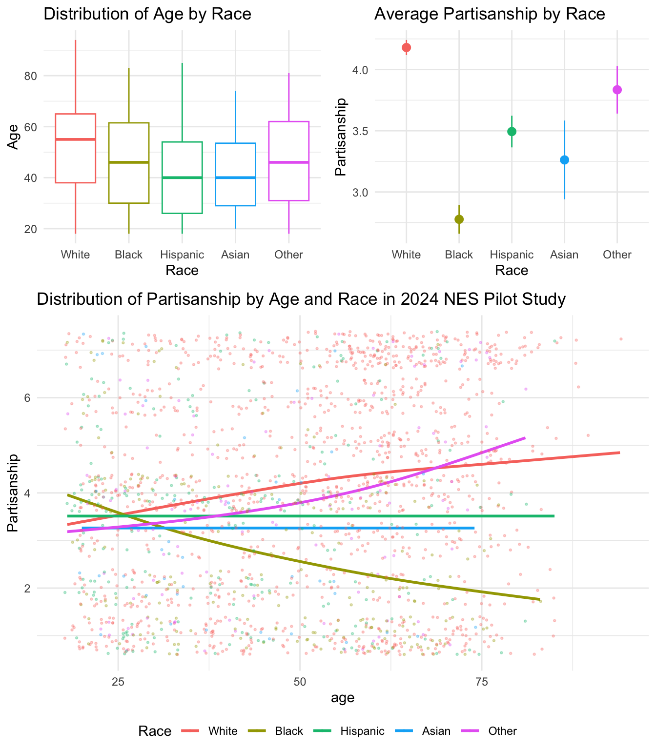
From the figure, we see that whites in sample have the highest median age (55 years) followed by Blacks (46 years). Hispanic and Asian respondents have the youngest median age of (40 years). Whites are also tend to lean more Republican in their partisanship than other racial minority groups. This is particularly true for older whites in the sample. Interestingly, average partisanship stays roughly constant with age for Asians and Hispanics, but older Black respondents are more likely to identify as Democrats than younger Blacks, whose partisan identification is more independent.
Please produce your own figure and provide a similar interpretation of what it conveys.
Please take a moment, to formulate some research questions you could ask of these data:
ME: How does support for Trump in the 2024 election vary with age and race?
YOU:
ME: On average, I expect that older voters will be more supportive of Trump, but suspect that this trend varies by race. I expect it will be particularly true among White voters, but less so among people of color. Since, partisanship is likely to be strong predictor of vote choice, I will explore whether these specific relationships hold, once we control for variations in partisan identification which we know varies both by age and race.
YOU:
ME:
I will estimate the following models:
\[
y = \beta_0 + \beta_1 age + \sum\beta_k race_k + \epsilon
\] If my expectations hold, I expect the coefficient on age in this model to be positive, indicating older voters are more likely to vote for Trump. White respondents are the reference category in this model4 and so the coefficients on the racial indicators (\(\beta_k race\)) correspond to how members of each racial group differ from white respondents in their propensity to vote for Trump. I expect all of these coefficients to be negative.
To explore whether the relationship between age and vote choice varies by race, I will fit an interaction model:
\[ y = \beta_0 + \beta_1 age + \sum\beta_k race_k + \epsilon + \sum\beta_{jk} age \times race_k + \epsilon \] This model allows the relationship between age and vote choice to vary by race. For white respondents, the relationship is described by \(\beta_1\). Again I expect it to be positive, suggesting older white voters are more likely to vote for trump. For racial minorities, the marginal effect of age for the racial or ethnic group \(k\) is described by \(\beta_1 + \beta_{jk}\). In general, I expect that the coefficients on \(\beta_{jk}\) to be negative such that older racial minorities are less likely to support Trump than older white respondents.
Finally, I will estimate a model that controls for partisanship. If the relationships between age, and race and vote choice are simply a reflection of differences in partisan identification, then coefficients on these predictors should no longer be statistically significant, while the coefficient on partisanship should positive and statistically significant.
\[ y = \beta_0 + \beta_1 pid + \beta_2 age + \sum\beta_k race_k + \epsilon + \sum\beta_{jk} age \times race_k \epsilon \]
You:
We will estimate the following models:
\[ y = \beta_0 + \beta_1 ... \]
\[ y = \beta_0 + \beta_1 ... \]
Below I estimate the three models described above
# Fit models
m1 <- lm_robust(dv_vote_trump2024 ~ age + race_5cat, df)
m2 <- lm_robust(dv_vote_trump2024 ~ age*race_5cat, df)
m3 <- lm_robust(dv_vote_trump2024 ~ age*race_5cat + partyid, df)Please produce
Interpret your results using both confidence intervals and hypothesis tests to assess the statistical significance of your claims and predicted values to help interpret the substantive significance of your results
htmlreg(list(m1, m2, m3),
        custom.model.names = c(
          "Baseline", "Interaction", "Alternative"
        ),
        caption = "Support for Trump in 2024",
        caption.above = T,
        custom.coef.names = c(
          "(Intercept)",
          "Age",
          "Black",
          "Hispanic",
          "Asian",
          "Other",
          "Age:Black",
          "Age:Hispanic",
          "Age:Asian",
          "Age:Other",
          "Party ID"
        ) ,
        include.ci = F,
digits = 3)| Baseline | Interaction | Alternative | |
|---|---|---|---|
| (Intercept) | 0.449*** | 0.361*** | -0.160*** |
| (0.038) | (0.045) | (0.032) | |
| Age | 0.002** | 0.004*** | -0.000 |
| (0.001) | (0.001) | (0.001) | |
| Black | -0.280*** | 0.213* | -0.038 |
| (0.034) | (0.100) | (0.083) | |
| Hispanic | -0.089* | 0.045 | -0.052 |
| (0.038) | (0.101) | (0.073) | |
| Asian | -0.238** | 0.007 | -0.233 |
| (0.076) | (0.236) | (0.136) | |
| Other | -0.031 | -0.035 | 0.125 |
| (0.052) | (0.152) | (0.108) | |
| Age:Black | -0.011*** | -0.000 | |
| (0.002) | (0.002) | ||
| Age:Hispanic | -0.003 | 0.001 | |
| (0.002) | (0.001) | ||
| Age:Asian | -0.005 | 0.003 | |
| (0.005) | (0.003) | ||
| Age:Other | 0.000 | -0.002 | |
| (0.003) | (0.002) | ||
| Party ID | 0.173*** | ||
| (0.003) | |||
| R2 | 0.047 | 0.061 | 0.569 |
| Adj. R2 | 0.044 | 0.056 | 0.566 |
| Num. obs. | 1735 | 1735 | 1691 |
| RMSE | 0.489 | 0.486 | 0.329 |
| ***p < 0.001; **p < 0.01; *p < 0.05 | |||
# Predictors for m2
pred_dfm2 <- expand_grid(
  age = seq(min(df$age, na.rm =T), max(df$age, na.rm = T)),
  race_5cat = sort(unique(df$race_5cat))
)

# Predictions with confidence intervals
pred_dfm2 <- cbind(
  pred_dfm2,
  predict(m2, newdata = pred_dfm2, interval = "confidence")$fit
)

# Plot predictions from m2

fig_m2 <- pred_dfm2 %>%
  ggplot(aes(age, fit, col = race_5cat))+
  geom_ribbon(aes(ymin = lwr, ymax = upr,
    fill = race_5cat
    ),
    alpha = .5)+
  geom_line()+
  facet_wrap( ~ race_5cat)+
  theme_minimal()+
  guides(
    col = "none",
    fill = "none"
  )+
  labs(
    y = "Predicted Vote Choice",
    title = "Support for Trump by Age and Race"
  )

# Display figure
fig_m2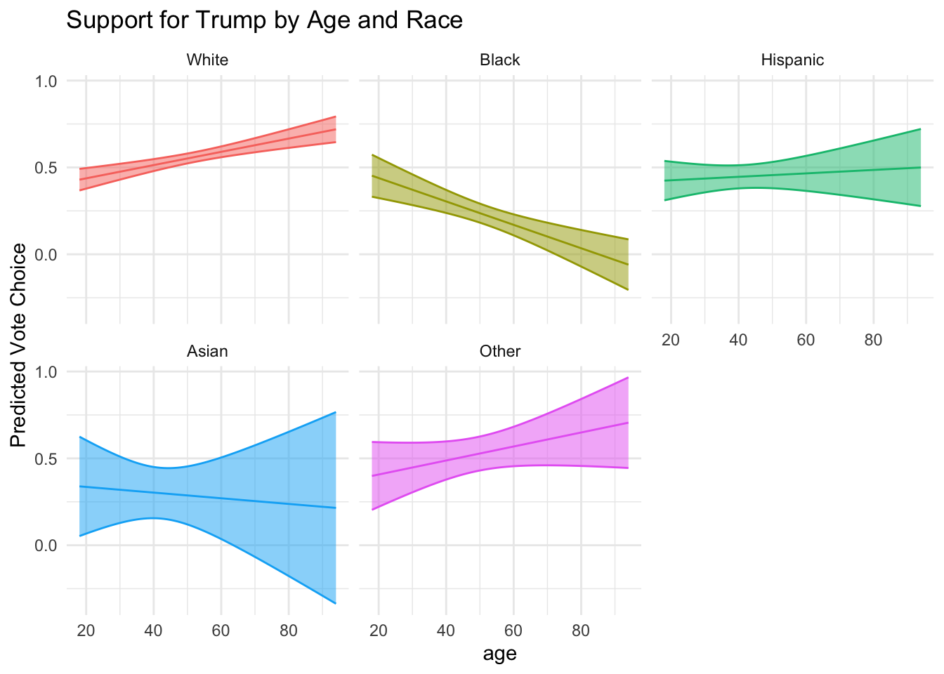
# Predictors for m3
pred_dfm3 <- expand_grid(
  age = seq(min(df$age, na.rm =T), max(df$age, na.rm = T)),
  race_5cat = sort(unique(df$race_5cat)),
  partyid = mean(df$partyid, na.rm=T)
)

# Predictions with confidence intervals
pred_dfm3 <- cbind(
  pred_dfm3,
  predict(m3, newdata = pred_dfm3, interval = "confidence")$fit
)

# Plot predictions from m2

fig_m3 <- pred_dfm3 %>%
  ggplot(aes(age, fit, col = race_5cat))+
  geom_ribbon(aes(ymin = lwr, ymax = upr,
    fill = race_5cat
    ),
    alpha = .5)+
  geom_line()+
  facet_wrap( ~ race_5cat)+
  theme_minimal()+
  guides(
    col = "none",
    fill = "none"
  )+
  labs(
    y = "Predicted Vote Choice",
    title = "Support for Trump by Age and Race Controlling for Partisanship"
  )

fig_m3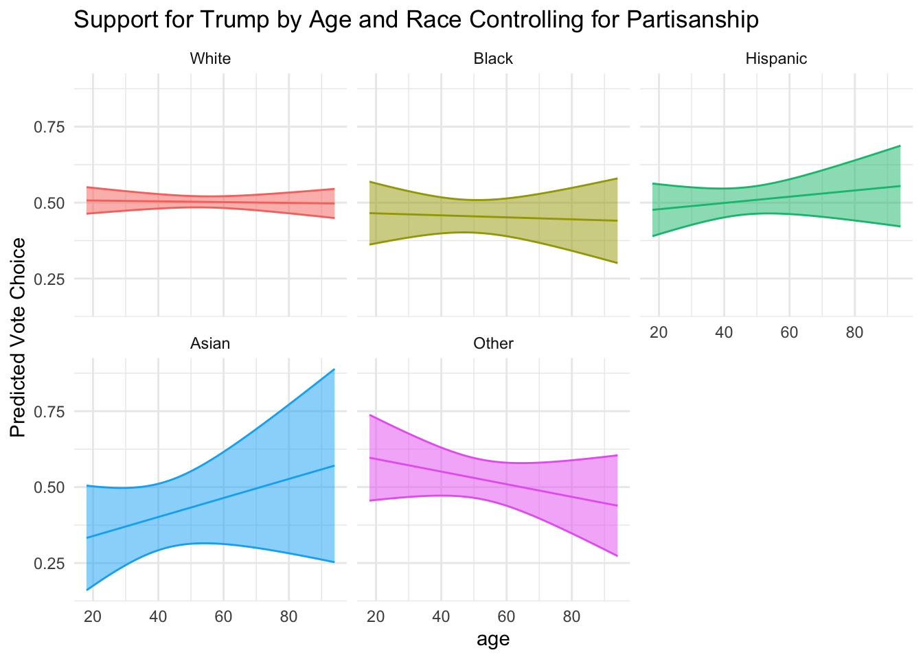
ME: Our baseline model confirms our initial expectations. Controlling for race, older respondents have higher predicted levels of support for Trump by 0.002 percentage points. Controlling for race, the model predicts that a 60 year old respondent is about 6.3 percentage points more likely to vote for Trump than a 30 year-old respondent. The test statistic for this coefficient is 3.10 corresponding to a p-value < 0.05, suggesting that if there were no relationship between age and vote choice in this model, it would be very unlikely that we observed a test statistic of this magnitude. Similarly the confidence interval for this estimate has suggests that coefficients as small as 0.0008 and as large as 0.0034 are plausible values for the relationship between age and vote choice in these data. Similarly, controlling for age, Black, Hispanic, and Asian respondents report significantly lower levels of support for Trump than white respondents (p < 0.05).
Turning to the interaction model, we see that the magnitude of the coefficient on age (which corresponds to the marginal effect of age for white respondents) increases, while the coefficients on the interactions between age and racial indicators are generally negative, suggesting that the relationship between age and support for Trump is less strong for these racial and ethnic groups. Figure 1 helps clarify these marginal effects, as we see that slope for age is clearly positive for white respondents, clearly negative for Black respondents. The confidence intervals for the predicted values of the other racial and ethnic groups are generally wide, and consisent with positive, negative, or no relationship between age and vote choice.
Finally, looking at the model controlling for partisanship, we see that none of the relationships between age, race, and vote choice, remain statistically significant once we account for the relationships between partisanship and vote choice, and the relationships between partisanship and age and race. In sum, apparent demographic differences in support for Trump appear driven by the differences in partisan identification across racial groups and within age groups.
YOU:
In general, I try not to recode the original variables, but instead create new columns, with different names. But, like this footnote, it seems overly verbose to create something like age_recoded, so I’ll break my general rule↩︎
See note below↩︎
Which is the best kind of speaking↩︎
Because white is first level the factor variable race↩︎