# Define Population
N <- 10000
set.seed(123)
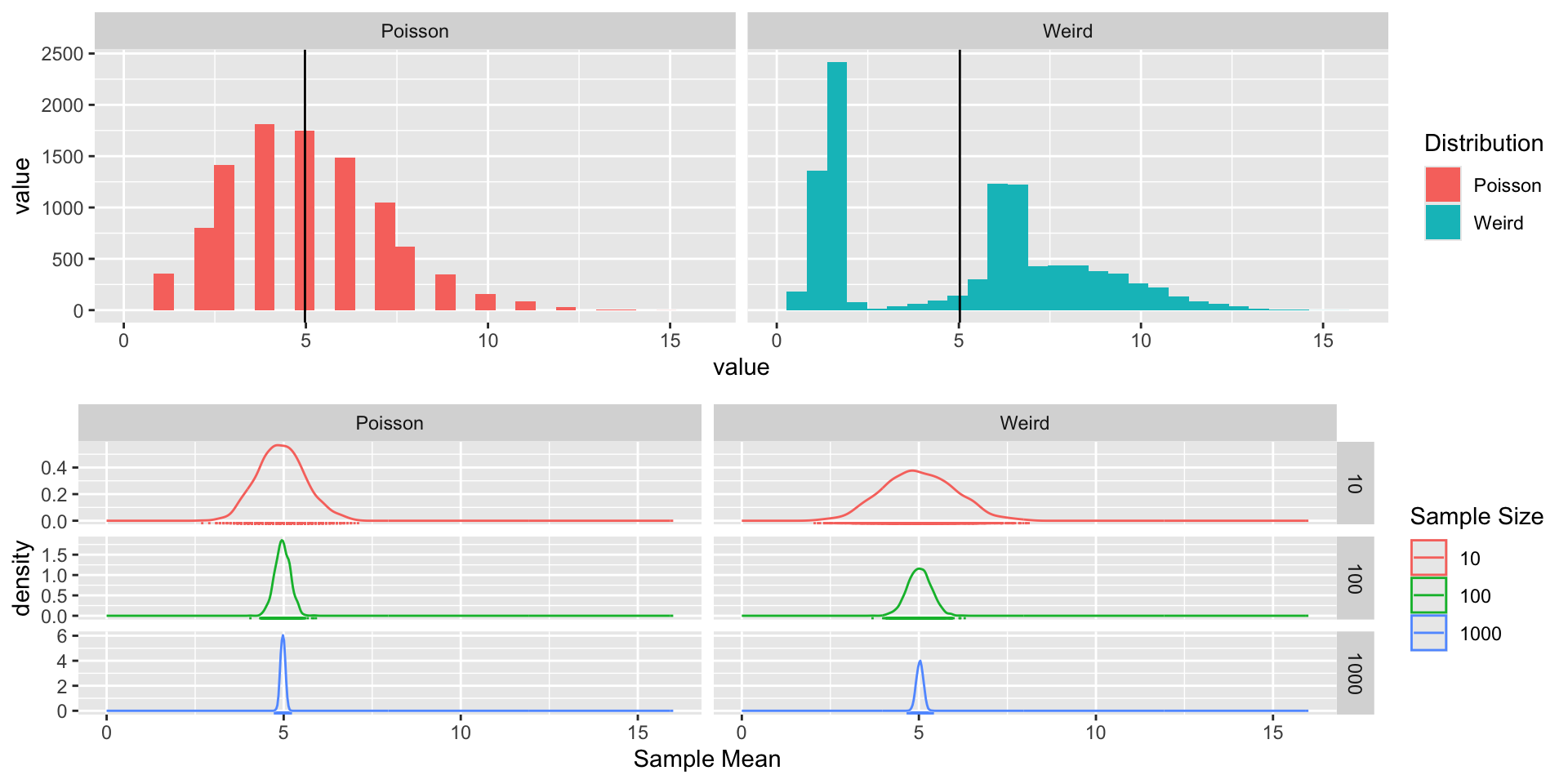
pop_df <- tibble(
Poisson = rpois(N, 5),
# Binomial = rbinom(size=20, n=N, prob = .25),
type = sample(0:2,N,replace =T,prob=c(.4,.2,.4)),
Weird = case_when(
type == 0 ~ rbeta(N,5,2)*2,
type == 1 ~ (rexp(N,4)-6.5)*-1,
type == 2 ~ rnorm(N,8,2)
)
) %>% select(Poisson, Weird)
fig_pop_dist <- pop_df %>%
pivot_longer(
col = everything(),
names_to = "Distribution"
) %>%
ggplot(aes(value,fill=Distribution,group=Distribution))+
geom_histogram()+
xlim(0,16)+
facet_grid(~Distribution,scales = "free_x")+
stat_summary(aes(x=0, y=value),fun.data =\(x) data.frame(xintercept = mean(x)), geom="vline")
sample_sizes <- c(10,100,1000)
calculate_sample_mean <- function(n,pop){
df <- tibble(
size = n,
`Sample Mean` = mean(sample(pop,n,replace = F))
)
return(df)
}
simulate_clt_fn <- function(nsims = 100, the_pop,the_n, ...){
sim <- 1:nsims %>% purrr::map_df(\(x)calculate_sample_mean(pop=the_pop, n=the_n))
return(sim)
}
# binomial_clt <- sample_sizes %>%
# purrr::map_df( \(x) simulate_clt_fn(nsims= 2000,the_pop = pop_df$Binomial, the_n = x)) %>%
# mutate(
# id = 1:n(),
# Distribution = "Binomial"
# )
poisson_clt <- sample_sizes %>%
purrr::map_df( \(x) simulate_clt_fn(nsims= 2000,the_pop = pop_df$Poisson, the_n = x)) %>%
mutate(
id = 1:n(),
Distribution = "Poisson"
)
weird_clt <- sample_sizes %>%
purrr::map_df( \(x) simulate_clt_fn(nsims= 2000,the_pop = pop_df$Weird, the_n = x)) %>%
mutate(
id = 1:n(),
Distribution = "Weird"
)
sample_df <- poisson_clt %>% bind_rows(weird_clt) %>%
mutate(
`Sample Size` = factor(size)
)
fig_samp_dist <- sample_df %>%
ggplot(aes(`Sample Mean`,col=`Sample Size`))+
geom_density()+
geom_rug()+
# theme( strip.background.y = element_blank(),
# strip.text.y = element_blank())+
xlim(0,16)+
facet_grid(`Sample Size`~Distribution,scales = "free_y")
fig_clt <- ggarrange(fig_pop_dist,fig_samp_dist,ncol=1)
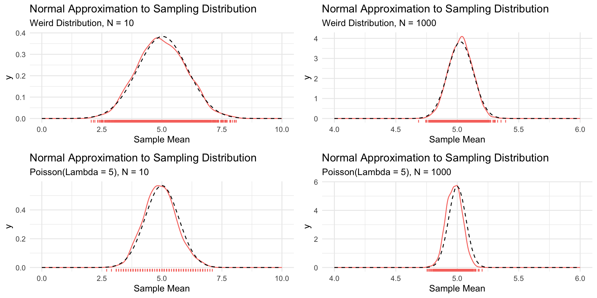
p10_weird <- sample_df %>%
filter(Distribution == "Weird") %>%
filter(size == 10) %>%
ggplot(aes(`Sample Mean`))+
geom_density(aes(col="Sample Size =10"))+
geom_rug(aes(col="Sample Size =10"))+
stat_function(
fun=dnorm, args = list(mean=mean(pop_df$Weird), sd=sd(pop_df$Weird)/sqrt(10)),
col="black",linetype = "dashed"
)+
xlim(0,10)+
theme_minimal()+
guides(col="none")+
labs(
title = "Normal Approximation to Sampling Distribution",
subtitle = "Weird Distribution, N = 10"
)
p1000_weird <- sample_df %>%
filter(Distribution == "Weird") %>%
filter(size == 1000) %>%
ggplot(aes(`Sample Mean`))+
geom_density(aes(col="Sample Size =1000"))+
geom_rug(aes(col="Sample Size =1000"))+
stat_function(
fun=dnorm, args = list(mean=mean(pop_df$Weird), sd=sd(pop_df$Weird)/sqrt(1000)),
col="black",linetype = "dashed"
)+
xlim(4,6)+
theme_minimal()+
guides(col="none")+
labs(
title = "Normal Approximation to Sampling Distribution",
subtitle = "Weird Distribution, N = 1000"
)
p10_poisson <- sample_df %>%
filter(Distribution == "Poisson") %>%
filter(size == 10) %>%
ggplot(aes(`Sample Mean`))+
geom_density(aes(col="Sample Size =10"))+
geom_rug(aes(col="Sample Size =10"))+
stat_function(
fun=dnorm, args = list(mean=5, sd=sd(pop_df$Poisson)/sqrt(10)),
col="black",linetype = "dashed"
)+
xlim(0,10)+
theme_minimal()+
guides(col="none")+
labs(
title = "Normal Approximation to Sampling Distribution",
subtitle = "Poisson(Lambda = 5), N = 10"
)
p1000_poisson <- sample_df %>%
filter(Distribution == "Poisson") %>%
filter(size == 1000) %>%
ggplot(aes(`Sample Mean`))+
geom_density(aes(col="Sample Size =1000"))+
geom_rug(aes(col="Sample Size =1000"))+
stat_function(
fun=dnorm, args = list(mean=5, sd=sd(pop_df$Poisson)/sqrt(1000)),
col="black",linetype = "dashed"
)+
xlim(4,6)+
theme_minimal()+
guides(col="none")+
labs(
title = "Normal Approximation to Sampling Distribution",
subtitle = "Poisson(Lambda = 5), N = 1000"
)
fig_clt_approx <- ggarrange(p10_weird, p1000_weird, p10_poisson,p1000_poisson)