POLS 2580

Statistical Inference
and Final Paper

Updated Dec 4, 2025

Overview

Class Plan

  • Announcements
  • Statistical Inference
  • Instrumental variables
  • Course Review
  • Final Projects

Setup: Packages for today

## Pacakges for today
the_packages <- c(
  ## R Markdown
  "tinytex", "kableExtra","DT","texreg","htmltools",
  ## Tidyverse
  "tidyverse", "lubridate", "forcats", "haven", "labelled",
  ## Extensions for ggplot
  "ggmap","ggrepel", "ggridges", "ggthemes", "ggpubr", 
  "patchwork",
  "GGally", "scales", "dagitty", "ggdag", "ggforce",
  # Data 
  "COVID19","maps","mapdata","qss","tidycensus", "dataverse", 
  # Analysis
  "DeclareDesign", "easystats", "zoo"
)

## Define a function to load (and if needed install) packages

ipak <- function(pkg){
    new.pkg <- pkg[!(pkg %in% installed.packages()[, "Package"])]
    if (length(new.pkg)) 
        install.packages(new.pkg, dependencies = TRUE)
    sapply(pkg, require, character.only = TRUE)
}

## Install (if needed) and load libraries in the_packages
ipak(the_packages)
      tinytex    kableExtra            DT        texreg     htmltools 
         TRUE          TRUE          TRUE          TRUE          TRUE 
    tidyverse     lubridate       forcats         haven      labelled 
         TRUE          TRUE          TRUE          TRUE          TRUE 
        ggmap       ggrepel      ggridges      ggthemes        ggpubr 
         TRUE          TRUE          TRUE          TRUE          TRUE 
    patchwork        GGally        scales       dagitty         ggdag 
         TRUE          TRUE          TRUE          TRUE          TRUE 
      ggforce       COVID19          maps       mapdata           qss 
         TRUE          TRUE          TRUE          TRUE          TRUE 
   tidycensus     dataverse DeclareDesign     easystats           zoo 
         TRUE          TRUE          TRUE          TRUE          TRUE 

Sampling distributions and standard errors

Populations and samples

  • Population: All the cases from which you could have sampled

  • Parameter: A quantity or quantities of interest often generically called \(\theta\) (β€œtheta”). What we want to learn about our population

  • Sample: A (random) draw of observations from that population

  • Sample Size: The number of observations in your draw (without replacement)

Estimators, estimates, and statistics

  • Estimator: A rule for calculating an estimate of our parameter of interest.

  • Estimate: The value produced by some estimator for some parameter from some data. Often called \(\hat{\theta}\)

  • Unbiased estimators: \(E(\hat{\theta})=E(\theta)\) On average, the estimates produced by some estimator will be centered around the truth

  • Consistent estimates: \(\lim_{n\to \infty} \hat{\theta_N} = \theta\) As the sample size increases, the estimates from an estimator converge in probability to the parameter value

  • Statistic: A summary of the data (mean, regression coefficient, \(R^2\)). An estimator without a specified target of inference

Distrubtions and standard errors

  • Sampling Distribution: How some estimate would vary if you took repeated samples from the population

  • Standard Error: The standard deviation of the sampling distribution

  • Resampling Distribution: How some estimate would vary if you took repeated samples from your sample WITH REPLACEMENT

    • β€œSampling from our sample, as the sample was sampled from the population.”

Sampling distributions

  • Treat the 2024 NES pilot as the population

  • Take repeated samples of size N = 10, 30, 300

  • For each sample of size N, calculate the sample mean of age

  • Plot the distribution of sample means (i.e. the sampling distribution)

# Load Data
load(url("https://pols2580.paultesta.org/files/data/nes24.rda"))

# ---- Population ----

# Population average
mu_age <- mean(df$age, na.rm=T)
# Population standard deviation
sd_age <- sd(df$age, na.rm = T)

# ---- Function to Take Repeated Samples From Data ----

sample_data_fn <- function(
    dat=df, var=age, samps=1000, sample_size=10,
    resample = F){
  if(resample == F){
  df <- tibble(
  sim = 1:samps,
  distribution = "Sampling",
  size = sample_size,
  sample_from = "Population",
  pop_mean = dat %>% pull(!!enquo(var)) %>% mean(., na.rm=T),
  pop_sd = dat %>% pull(!!enquo(var)) %>% sd(., na.rm=T),
  se_asymp = pop_sd / sqrt(size),
  ll_asymp = pop_mean - 1.96*se_asymp,
  ul_asymp = pop_mean + 1.96*se_asymp,
) %>% 
  mutate(
    sample = purrr::map(sim, ~ slice_sample(dat %>% select(!!enquo(var)), n = sample_size, replace = F)),
    sample_mean = purrr::map_dbl(sample, \(x) x %>% pull(!!enquo(var)) %>% mean(.,na.rm=T)),
    ll = sample_mean - 1.96*sd(sample_mean),
    ul = sample_mean + 1.96*sd(sample_mean)
  )
  }
  if(resample == T){
    df <- tibble(
  sim = 1:samps,
  distribution = "Resampling",
  size = sample_size,
  sample_from = "Sample",
  pop_mean = dat %>% pull(!!enquo(var)) %>% mean(., na.rm=T),
  pop_sd = dat %>% pull(!!enquo(var)) %>% sd(., na.rm=T),
  se_asymp = pop_sd / sqrt(size),
  ll_asymp = pop_mean - 1.96*se_asymp,
  ul_asymp = pop_mean + 1.96*se_asymp,
) %>% 
  mutate(
    sample = purrr::map(sim, ~ slice_sample(dat %>% select(!!enquo(var)), n = sample_size, replace = T)),
    sample_mean = purrr::map_dbl(sample, \(x) x %>% pull(!!enquo(var)) %>% mean(.,na.rm=T))
  )
  }
  return(df)
}

# ---- Plot Single Distribution -----

plot_distribution <- function(the_pop,the_samp, the_var, ...){
  mu_pop <- the_pop %>% pull(!!enquo(the_var)) %>% mean(., na.rm=T)
  mu_samp <- the_samp %>% pull(!!enquo(the_var)) %>% mean(., na.rm=T)
  ll <- the_pop %>% pull(!!enquo(the_var)) %>% as.numeric() %>%  min(., na.rm=T)
  ul <- the_pop %>% pull(!!enquo(the_var)) %>% as.numeric() %>% max(., na.rm=T)
  p<- the_samp %>% 
    ggplot(aes(!!enquo(the_var)))+
    geom_density()+
    geom_rug()+
    theme_void()+
    geom_vline(xintercept = mu_samp, col = "red")+
    geom_vline(xintercept = mu_pop, col = "grey40",linetype = "dashed")+
    xlim(ll,ul)
  return(p)
}

# ---- Plot multiple distributions ----

plot_samples <- function(pop, x, variable,n_rows = 4, ...){
  sample_plots <- x$sample[1:(4*n_rows)] %>% 
  purrr::map( \(x) plot_distribution(the_pop=pop, the_samp = x, 
                                     the_var = !!enquo(variable)))
  p <- wrap_elements(wrap_plots(sample_plots[1:(4*n_rows)], ncol=4))
  return(p)
  
}

# ---- Plot Combined Figure ----

plot_figure_fn <- function(
    d=df, 
    v=age, 
    sim=1000, 
    size=10,
    rows = 4){
  # Population average
  mu <- d %>% pull(!!enquo(v)) %>% mean(., na.rm=T)
  sd <- d %>% pull(!!enquo(v)) %>% sd(., na.rm=T)
  se <- sd/sqrt(size)
  # Range
  ll <- d %>% pull(!!enquo(v)) %>% as.numeric() %>%  min(., na.rm=T)
  ul <- d %>% pull(!!enquo(v)) %>% as.numeric() %>% max(., na.rm=T)
  # Population standard deviation
  # Sample data
  samp_df <- sample_data_fn(dat=d, var = !!enquo(v), samps = sim, sample_size = size)
  # Plot Population
  p_pop <- d %>%
    ggplot(aes(!!enquo(v)))+
      geom_density(col ="grey60")+
      geom_rug(col = "grey60", )+
      geom_vline(xintercept = mu, col="grey40", linetype="dashed")+
      theme_void()+
      labs(title ="Population")+
      xlim(ll,ul)+
      theme(plot.title = element_text(hjust = 0))

  
  p_samps <- plot_samples(pop=d, x= samp_df,variable = !!enquo(v),
                          n_rows = rows)
  p_samps <- p_samps + 
    ggtitle(paste("Repeated samples of size N =",size,"from the population"))+
    theme(plot.title = element_text(hjust = 0.5), 
          plot.background = element_rect(
            fill = NA, colour = 'black', linewidth = 2)
          )
  
  
  p_dist <- samp_df %>% 
  ggplot(aes(sample_mean))+
  geom_density(col="red",aes(y= after_stat(ndensity)))+
  geom_rug(col="red")+
  geom_density(data = df, aes(!!enquo(v), y= after_stat(ndensity)),
               col="grey60")+
  geom_vline(xintercept = mu, col="grey40", linetype="dashed")+
  xlim(ll,ul)+
  theme_void()+
    labs(
      title = "Sampling Distribution"
    )+  theme(plot.title = element_text(hjust = 0))
  
  range_upper_df <- tibble(
  x = seq( ((ll+ul)/2 -5), ((ll+ul)/2 +5), length.out = 20),
  xend = seq(ll-5, ul+5, length.out = 20),
  y = rep(9, 20),
  yend = rep(1, 20)
)
p_upper <- range_upper_df %>% 
  ggplot(aes(x=x, xend = xend, y=y,yend=yend))+
  geom_segment(
    arrow = arrow(length = unit(0.05, "npc"))
  )+
  theme_void()+
  coord_fixed(ylim=c(0,10),
              xlim =c(ll-5,ul+5),clip="off")
  # Lower
  range_df <- samp_df %>% 
  summarise(
    min = min(sample_mean),
    max = max(sample_mean),
    mean = mean(sample_mean)
  )
  
  plot_df <- tibble(
  id = 1:50,
  # x = sort(rnorm(50, mu, sd)),
  x = sort(runif(50, ll, ul)),
  xend = sort(rnorm(50, mu, se)),
  y = 9,
  yend = 1
)

p_lower <- plot_df %>%
  ggplot(aes(x,y, group =id))+
  geom_segment(aes(xend=xend, yend=yend),
               col = "red",arrow = arrow(length = unit(0.05, "npc"))
               )+
  theme_void()+
  coord_fixed(ylim=c(0,10),xlim = c(ll,ul),clip="off")

  
  design <-"##AAAA##
            ##AAAA##
            ##AAAA##
            BBBBBBBB
            BBBBBBBB
            #CCCCCC#
            #CCCCCC#
            #CCCCCC#
            #CCCCCC#
            DDDDDDDD
            DDDDDDDD
            ##EEEE##
            ##EEEE##
            ##EEEE##"
  
  fig <- p_pop / p_upper / p_samps / p_lower / p_dist +
    plot_layout(design = design)
  return(fig)


}

# ---- Samples and Figures Varying Sample Size ----
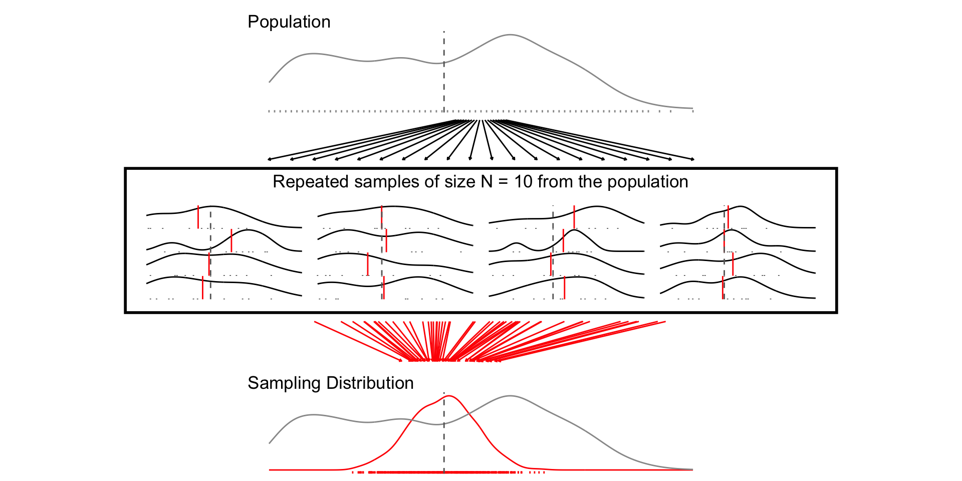
## N = 10
set.seed(1234)
samp_n10 <- sample_data_fn(sample_size  = 10, samps = 1000)
set.seed(1234)
fig_n10 <- plot_figure_fn(v=age,size = 10)
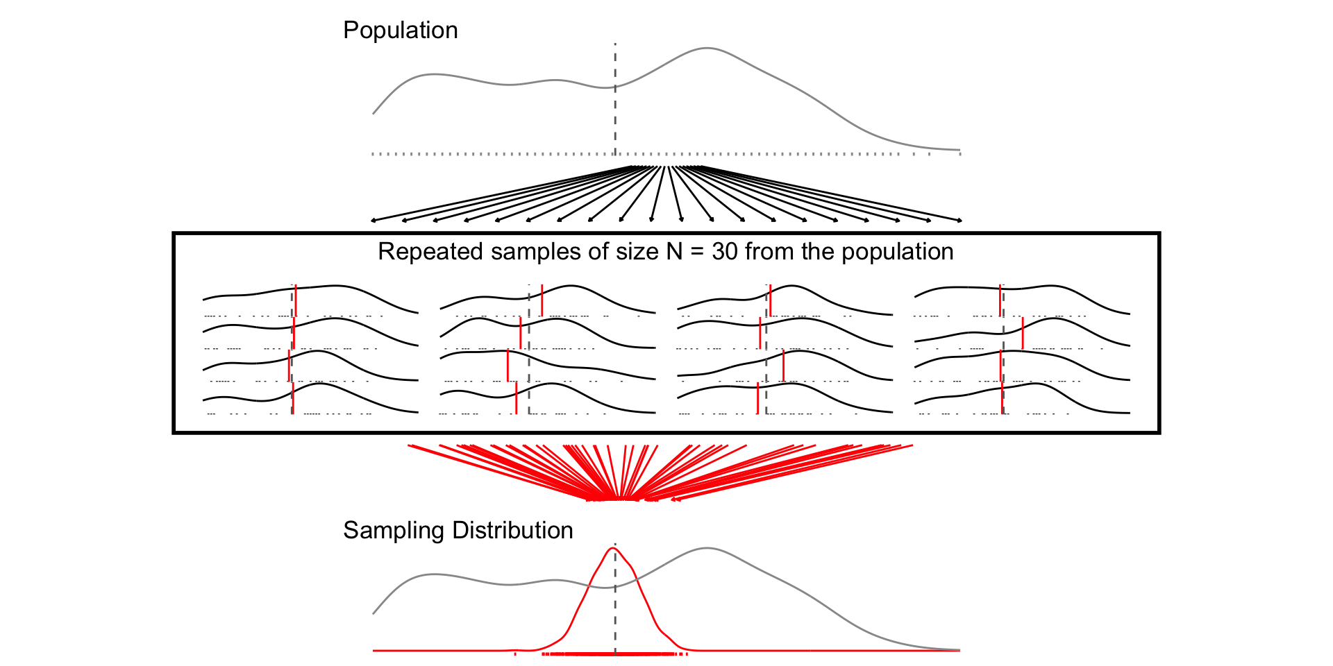
## N = 30
set.seed(1234)
samp_n30 <- sample_data_fn(sample_size  = 30, samps = 1000)
set.seed(1234)
fig_n30 <- plot_figure_fn(size = 30,rows=4)
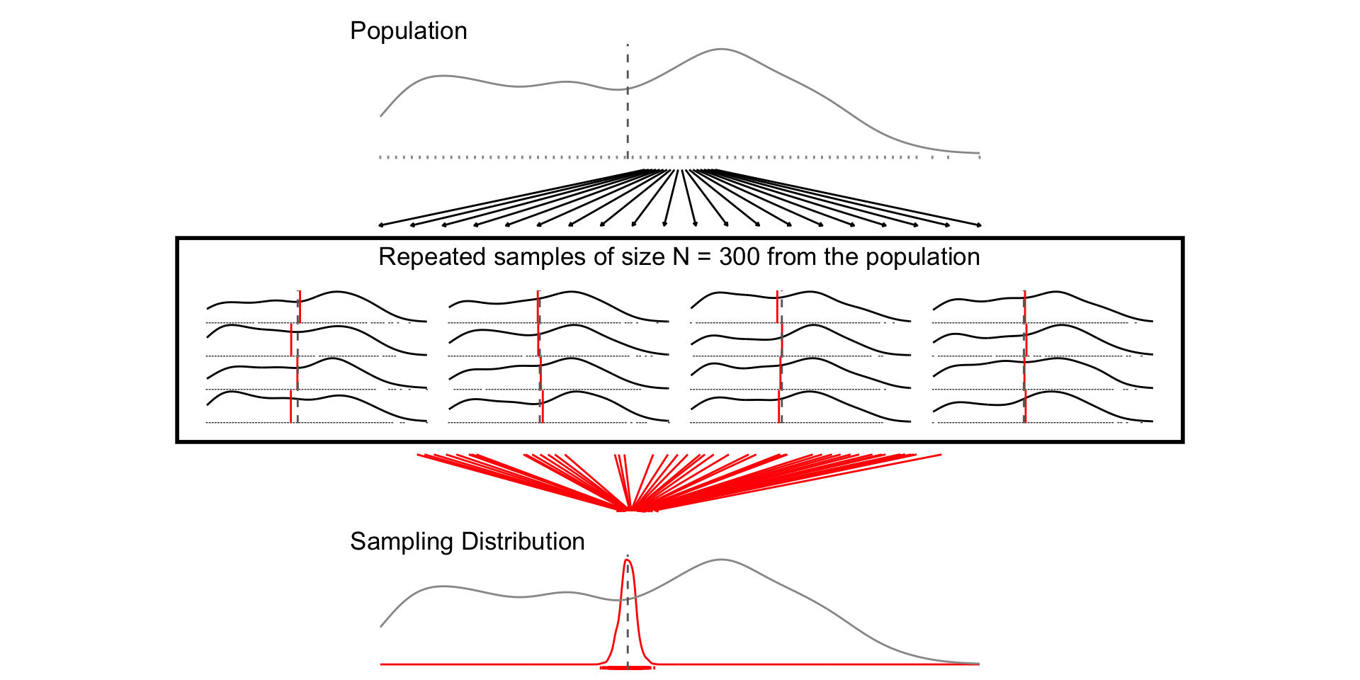
## N = 300
set.seed(1234)
samp_n300 <- sample_data_fn(sample_size  = 300, samps = 1000)
set.seed(1234)
fig_n300 <- plot_figure_fn(size = 300)

As the sample sample size increases:

  • The width of the sampling distribution decreases (LLN)

  • The shape of the sampling distribution approximates a Normal distribution (CLT)

Standard errors

  • The standard error (SE) is simply the standard deviation of the sampling distribution.

  • The SE decreases as the sample size increases (by the LLN):

  • Approximately 95% of the sample means will be within 2 SEs of the population mean (CLT)

se_df <- tibble(
  `Sample Size` = factor(paste("N =",c(10,30, 300))),
  se = c(sd(samp_n10$sample_mean),
         sd(samp_n30$sample_mean),
         sd(samp_n300$sample_mean)),
  SE = paste("SE =", round(se,2)),
  ll = mu_age,
  ul = mu_age + se,
  y = c(.3,.3,.45),
  yend = y
)

ci_df <- tibble(
  `Sample Size` = factor(paste("N =",c(10,30, 300))),
  se = c(sd(samp_n10$sample_mean),
         sd(samp_n30$sample_mean),
         sd(samp_n300$sample_mean)),
  mu = mu_age,
  ll = round(mu_age - 1.96 *se,2),
  ul = round(mu_age + 1.96 *se,2),
  ci = paste("95 % Coverage Interval [",ll,";",ul,"]",sep=""),
  y = c(.3,.3,.45),
  yend = y
)
sim_df <- samp_n10 %>% 
  bind_rows(samp_n30) %>% 
  bind_rows(samp_n300) %>% 
  mutate(
    `Sample Size` = factor(paste("N =",size))
    ) %>% 
  left_join(ci_df) %>% 
  mutate(
    Coverage = case_when(
      sample_mean > ll_asymp & sample_mean < ul_asymp  & size == 10~ "#F8766D",
      sample_mean > ll_asymp & sample_mean < ul_asymp  & size == 30~ "#00BA38",
      sample_mean > ll_asymp & sample_mean < ul_asymp  & size == 300~ "#619CFF",
      T ~ "grey"
    )
  )


fig_se <- sim_df %>% 
  ggplot(aes(sample_mean, col = `Sample Size`))+
  geom_density()+
  geom_rug()+
  geom_vline(xintercept = mu_age, linetype = "dashed")+
  theme_minimal()+
  facet_wrap(~`Sample Size`, ncol=1)+
  ylim(0,.5)+
  guides(col="none")+
  geom_segment(
    data = se_df,
    aes(x= ll, xend =ul, y = y, yend = yend)
  )+
  geom_text(
    data = se_df,
    aes(x = ul, y =y, label = SE),
    hjust = -.25
  ) +
  labs(
    y = "",
    x = "Sampling Distributions of Sample Means",
    title = "Standard Errors decrease with Sample Size"
  )

fig_coverage <- sim_df %>% 
  ggplot(aes(sample_mean,col=`Sample Size`))+
  geom_density()+
  geom_rug(col=sim_df$Coverage)+
  geom_vline(xintercept = mu_age, linetype = "dashed")+
  theme_minimal()+
  facet_wrap(~`Sample Size`, ncol=1)+
  ylim(0,.55)+
  guides(col="none")+
  geom_segment(
    data = ci_df,
    aes(x= ll, xend =ul, y = y, yend = yend)
  )+
  geom_text(
    data = ci_df,
    aes(x = mu, y =y, label = ci),
    hjust = .5,
    nudge_y =.1
  ) +
  labs(
    y = "",
    x = "Sampling Distributions of Sample Means",
    title = "Approximately 95% of sample means are within 2 SE of the population mean"
  )

How do we calculate a standard error from a single sample?

Calculating standard errors

  • Simulation:
    • Treat sample as population
    • Sample with replacement (β€œbootstrapping”)
    • Estimate SE from standard deviation of resampling distribution (β€œplug-in principle”)
  • Analytic
    • Characterize sampling distribution from sample mean and variance via asymptotic theory (the LLT and CLT)
    • For a sample mean, \(\bar{x}\)

\[ SE_{\bar{x}} = \frac{\sigma_x}{\sqrt(n)} \]

plot_resampling_fn <- function(d=df, v=age, sim=1000, size=10,rows=3){
  # Population average
  mu <- d %>% pull(!!enquo(v)) %>% mean(., na.rm=T)
  # Population standard deviation and SE
  sd <- d %>% pull(!!enquo(v)) %>% sd(., na.rm=T)
  se <- sd/sqrt(size)
  # Range
  ll <- d %>% pull(!!enquo(v)) %>% as.numeric() %>%  min(., na.rm=T)
  ul <- d %>% pull(!!enquo(v)) %>% as.numeric() %>% max(., na.rm=T)
  # Resampling with replace
  # Draw 1 Sample
  sample <- sample_data_fn(dat=d, var = !!enquo(v), samps = 1, sample_size = size, resample = F)
  samp_df <- as.data.frame(sample$sample)
  # Resample from sample with replacement
  resamp_df <- sample_data_fn(dat=samp_df, var = !!enquo(v), samps = sim, sample_size = size, resample = T)
  # Plot Population
  p_pop <- d %>%
    ggplot(aes(!!enquo(v)))+
      geom_density(col ="grey60")+
      geom_rug(col = "grey60", )+
      geom_vline(xintercept = mu, col="grey40", linetype="dashed")+
      theme_void()+
      labs(title ="Population")+
      xlim(ll,ul)+
      theme(plot.title = element_text(hjust = 0))

  p_samp <- plot_distribution(the_pop = d,
                              the_samp = samp_df,
                              the_var = age)+
    labs(title ="Sample")+
      xlim(ll,ul)+
      theme(plot.title = element_text(hjust = 0))
  
  p_samps <- plot_samples(pop=d, x= resamp_df,variable = !!enquo(v), n_rows =rows)
  p_samps <- p_samps + 
    ggtitle(paste("Repeated samples with replacement\nof size N =",size,"from sample"))+
    theme(plot.title = element_text(hjust = 0.5), 
          plot.background = element_rect(
            fill = NA, colour = 'black', linewidth = 2)
          )
  
  # Resampling Distribution
  
  
  p_dist <- resamp_df %>% 
  ggplot(aes(sample_mean))+
  geom_density(col="red",aes(y= after_stat(ndensity)))+
  geom_rug(col="red")+
  geom_density(data = df, aes(!!enquo(v), y= after_stat(ndensity)),
               col="grey60")+
  geom_vline(xintercept = unique(resamp_df$pop_mean), col="red", linetype="solid")+
  geom_vline(xintercept = mu, col="grey40", linetype="dashed")+
  xlim(ll,ul)+
  theme_void()+
    labs(
      title = "Reampling Distribution"
    )+  theme(plot.title = element_text(hjust = 0))
  
   range_upper_df <- tibble(
  x = seq( ((ll+ul)/2 -5), ((ll+ul)/2 +5), length.out = 20),
  xend = seq(ll-5, ul+5, length.out = 20),
  y = rep(9, 20),
  yend = rep(1, 20)
)
p_upper <- range_upper_df %>% 
  ggplot(aes(x=x, xend = xend, y=y,yend=yend))+
  geom_segment(
    arrow = arrow(length = unit(0.05, "npc"))
  )+
  theme_void()+
  coord_fixed(ylim=c(0,10),
              xlim =c(ll-5,ul+5),clip="off")
  # Lower
  range_df <- resamp_df %>% 
  summarise(
    min = min(sample_mean),
    max = max(sample_mean),
    mean = mean(sample_mean)
  )
  
  plot_df <- tibble(
  id = 1:50,
  # x = sort(rnorm(50, mu, sd)),
  x = sort(runif(50, ll, ul)),
  xend = sort(rnorm(50, unique(resamp_df$pop_mean), se)),
  y = 9,
  yend = 1
)

p_lower <- plot_df %>%
  ggplot(aes(x,y, group =id))+
  geom_segment(aes(xend=xend, yend=yend),
               col = "red",arrow = arrow(length = unit(0.05, "npc"))
               )+
  theme_void()+
  coord_fixed(ylim=c(0,10),xlim = c(ll,ul),clip="off")

  
  design <-"##AAAA##
            ##AAAA##
            ##AAAA##
            ##BBBB##
            ##BBBB##
            ##BBBB##            
            CCCCCCCC
            CCCCCCCC
            #DDDDDD#
            #DDDDDD#
            #DDDDDD#
            #DDDDDD#
            EEEEEEEE
            EEEEEEEE
            ##FFFF##
            ##FFFF##
            ##FFFF##"
  
  fig <- p_pop / p_samp /p_upper / p_samps / p_lower / p_dist +
    plot_layout(design = design)
  return(fig)


}
set.seed(123)
resamp_n10 <- sample_data_fn(
  dat = sample_data_fn(samps = 1, sample_size = 10, resample = T)$sample %>%  as.data.frame(),
  sample_size = 10, 
  resample = T)
set.seed(123)
fig_n10_bs <- plot_resampling_fn(size=10)

set.seed(12345)
resamp_n30 <- sample_data_fn(
  dat = sample_data_fn(samps = 1, sample_size = 30, resample = T)$sample %>%  as.data.frame(),
  samps = 1000, sample_size = 30, resample = T)

set.seed(12345)
fig_n30_bs <- plot_resampling_fn(size=30)

set.seed(1234)
resamp_n300 <- sample_data_fn(
  dat = sample_data_fn(samps = 1, sample_size = 300, resample = T)$sample %>%  as.data.frame(),
  samps = 1000, sample_size = 300, resample = T)
set.seed(1234)
fig_n300_bs <- plot_resampling_fn(size=300)

Bootstrap SE Analytic SE
5.74 5.61
2.75 3.24
1.07 1.02

Confidence intervals

Confidence intervals

Confidence intervals:

  • provide a way of quantifying uncertainty about estimates

  • describe a range of plausible values for an estimate

  • are a function of the standard error of the estimate, and the a critical value determined by \(\alpha\), which describes the degree of confidence we want

Calculating a confidence interval

  • Choose level of confidence \((1-\alpha)\times 100%\)

    • \(\alpha = 0.05\), corresponds to a 95% confidence level.
  • Derive the sampling distribution of the estimator

    • Simulation: bootstrap re-sampling
    • Analytically: computing its mean and variance.
  • Compute the standard error

  • Compute the critical value \(z_{\alpha/2}\)

    • as the \(1.96 = \Phi(z_{0.5/2})\) for a 95% CI
  • Compute the lower and upper confidence limits

    • lower limit = \(\hat{\theta} - z_{\alpha/2}\times SE\)
    • upper limit = \(\hat{\theta} + z_{\alpha/2}\times SE\)
resamp_df <- 
  resamp_n10 %>% 
  bind_rows(resamp_n30) %>% 
  bind_rows(resamp_n300) %>% 
  mutate(
    `Sample Size` = factor(paste("N =",size))
    )

resamp_ci_df <- tibble(
  `Sample Size` = factor(paste("N =",c(10,30,300))),
  mu = unique(resamp_df$pop_mean),
  ll = unique(resamp_df$ll_asymp),
  ul = unique(resamp_df$ul_asymp),
  y = c(.3, .3,.5)
)

fig_ci1 <- resamp_df %>% 
  ggplot(aes(sample_mean,
             col = `Sample Size`))+
  geom_density()+
  geom_rug()+
  geom_vline(xintercept = mu_age, linetype = "dashed")+
  geom_vline(data = resamp_ci_df,
             aes(xintercept = mu,
                 col = `Sample Size`))+
  geom_segment(data = resamp_ci_df,
               aes(x = ll, xend =ul, y = y, yend =y,
                   col = `Sample Size`))+
  facet_wrap(~`Sample Size`, ncol=1)+
  theme_minimal()+
  labs(
    y = "",
    x = "Resampling Distribution",
    title = "95% Confidence Intervals"
  )
  

samp_ci_df <- samp_n10 %>% 
  bind_rows(samp_n30) %>% 
  bind_rows(samp_n300) %>% 
  mutate(
    `Sample Size` = factor(paste("N =",size))
    ) %>% 
  mutate(
    Coverage = case_when(
      pop_mean > ll & pop_mean < ul ~ "red",
      T ~ "black"
    )
  )

fig_ci2 <- samp_ci_df %>% 
  filter(sim %in% 1:100) %>% 
  filter(size == 10) %>% 
  ggplot(aes(y = sample_mean, x= sim))+
  geom_pointrange(aes(ymin = ll, ymax =ul, col=Coverage))+
  geom_hline(yintercept = mu_age, linetype = "dashed")+
  coord_flip()+
  theme_minimal()+
  guides(col = "none")+
  facet_wrap(~`Sample Size`)

fig_ci3 <- samp_ci_df %>% 
  filter(sim %in% 1:100) %>% 
  ggplot(aes(y = sample_mean, x= sim))+
  geom_pointrange(aes(ymin = ll, ymax =ul, col=Coverage))+
  geom_hline(yintercept = mu_age, linetype = "dashed")+
  coord_flip()+
  theme_minimal()+
  guides(col = "none")+
  facet_wrap(~`Sample Size`)

  • Figure 1 shows 3 confidences intervals for 3 samples of different sizes (N = 10, 30, 300). The CIs for N = 10 and N = 300, intervals contain the truth (include the population mean). By chance, the CI for N=30 falls outside of the truth.

  • Figure 2 shows that our confidence is about the property of the interval. Over repeated sampling, 95% of the intervals would contain the truth, 5% percent would not.

    • In any one sample, the population parameter either is or is not within the interval.
  • Figure 3, shows that while the width of the interval declines with the sample size, the coverage properties remains the same.

Interpreting confidence intervals

  • A confidence interval is constructed by a procedure that, in repeated samples, covers the true parameter with probability 95%.

    • \(\alpha = 0.05\) corresponds to a β€œ95-percent confidence interval”
  • Our β€œconfidence” is about the interval

  • In repeated sampling, we expect that \((1-\alpha) \times 100\%\) of the intervals we construct would contain the truth.

  • For any one interval, the truth, \(\theta\), either falls within in the lower and upper bounds of the interval or it does not.

Hypothesis testing

What is a hypothesis test

  • A formal way of assessing statistical evidence. Combines

    • Deductive reasoning distribution of a test statistic, if the a null hypothesis were true

    • Inductive reasoning based on the test statistic we observed, how likely is it that we would observe it if the null were true?

What is a test statistic?

  • A way of summarizing data
    • difference of means
    • coefficients from a linear model
    • coefficients from a linear model divided by their standard errors
    • R^2
    • Sums of ranks

Note

Different test statistics may be more or less appropriate depending on your data and questions.

What is a null hypothesis?

  • A statement about the world

    • Only interesting if we reject it

    • Would yield a distribution of test statistics under the null

    • Typically something like β€œX has no effect on Y” (Null = no effect)

    • Never accept the null can only reject

What is a p-value?

A p-value is a conditional probability summarizing the likelihood of observing a test statistic as far from our hypothesis or farther, if our hypothesis were true.

How do we do hypothesis testing?

  1. Posit a hypothesis (e.g. \(\beta = 0\))

  2. Calculate the test statistic (e.g. \((\hat{\beta}-\beta)/se_\beta\))

  3. Derive the distribution of the test statistic under the null via simulation or asymptotic theory

  4. Compare the test statistic to the distribution under the null

  5. Calculate p-value (Two Sided vs One sided tests)

  6. Reject or fail to reject/retain our hypothesis based on some threshold of statistical significance (e.g. p < 0.05)

Outcomes of hypothesis tests

  • Two conclusions from of a hypothesis test: we can reject or fail to reject a hypothesis test.

  • We never β€œaccept” a hypothesis, since there are, in theory, an infinite number of other hypotheses we could have tested.

Our decision can produce four outcomes and two types of error:

Reject \(H_0\) Fail to Reject \(H_0\)
\(H_0\) is true False Positive Correct!
\(H_0\) is false Correct! False Negative
  • Type 1 Errors: False Positive Rate (p < 0.05)
  • Type 2 Errors: False negative rate (1 - Power of test)

Quantifying uncertainty in regression

Quantifying uncertainty in regression

How do income and education shape political participation?

Let’s fit the following model

\[ y = \beta_0 + \beta_1\text{income} + \beta_2 \text{education} + \epsilon \]

m1 <- lm_robust(dv_participation ~   education + income, df)

And unpack the output

tidy(m1) %>% 
  mutate_if(is.numeric, \(x) round(x, 3)) -> m1_sum
m1_sum
         term estimate std.error statistic p.value conf.low conf.high   df
1 (Intercept)    0.312     0.080     3.910   0.000    0.155     0.468 1684
2   education    0.167     0.024     6.891   0.000    0.119     0.214 1684
3      income    0.007     0.010     0.671   0.502   -0.014     0.028 1684
           outcome
1 dv_participation
2 dv_participation
3 dv_participation
htmlreg(m1,include.ci=F) 
Statistical models
  Model 1
(Intercept) 0.31***
  (0.08)
education 0.17***
  (0.02)
income 0.01
  (0.01)
R2 0.04
Adj. R2 0.04
Num. obs. 1687
RMSE 1.29
***p < 0.001; **p < 0.01; *p < 0.05
htmlreg(m1,include.ci=T) 
Statistical models
  Model 1
(Intercept) 0.31*
  [ 0.16; 0.47]
education 0.17*
  [ 0.12; 0.21]
income 0.01
  [-0.01; 0.03]
R2 0.04
Adj. R2 0.04
Num. obs. 1687
RMSE 1.29
* 0 outside the confidence interval.
m1_coefplot <- m1_sum %>% 
  ggplot(aes(term, estimate))+
  geom_pointrange(aes(ymin = conf.low, ymax =conf.high))+
  geom_hline(yintercept = 0, linetype = "dashed")+
  coord_flip()+
  labs(
    y = "Estimate",
    x = "",
    title = "Coefficient plot"
  )+
  theme_minimal()

Estimates

The estimate column are the regression coefficients, \(\beta\)

Recall, lm_robust() calculates these:

\[ \hat{\beta} = (X'X)^{-1}X'y \]

Tip

\(\beta\)s describe substantive relationships between predictors (income, education) and the outcome (political participation)

coef(m1)
(Intercept)   education      income 
0.311609712 0.166755964 0.007034253 
X <- model.matrix(m1,data=df)
y <- model.frame(m1)$dv_participation
betas <- solve(t(X)%*%X)%*%t(X)%*%y
betas
                   [,1]
(Intercept) 0.311609712
education   0.166755964
income      0.007034253

A unit increases in education is associated with about 0.16 more acts of political participation, while a unit increase in income is associated with 0.007 more acts of participation.

Note that both income and education are measured with ordinal scales

get_value_labels(df$educ)
    No HS credential High school graduate         Some college 
                   1                    2                    3 
       2-year degree        4-year degree            Post-grad 
                   4                    5                    6 

Such that it might be unreasonable to assume cardinality (going from a 1 to 2 is the same as going from a 3 to 4)

  • Consider treating as factor / recoding variable

Standard errors & confidence intervals

The default standard errors from lm_robust() are calculated as follows

\[ SE_{\beta} = (X'X)^{-1}X'\text{diag}\left[\frac{e_i^2}{1-h_{ii}}\right]X(X'X)^{-1} \]

Which we could also obtain via bootstrapping.

The confidence intervals are calculated as follows:

\[ CI = \beta \pm 1.96\times SE_\beta \]

# 0 Set seed
set.seed(123)

# 1,000 bootstrap samples
boot <- modelr::bootstrap(df %>% select(dv_participation, income, education), 1000)
# Estimate Boostrapped Models
m1_bs <- purrr::map(boot$strap, ~ lm_robust(dv_participation ~  income + education, data = .))

# Tidy coefficients
m1_bs_df <- map_df(m1_bs, tidy, .id = "id")
m1_asymp_df <- tidy(m1) %>% 
  mutate(
    term = factor(term)
  ) %>% 
  select(term,estimate, std.error,conf.low, conf.high) %>% 
  mutate(
    ll = conf.low,
    ul = conf.high,
    y = 1.1,
    type = "Analytic"
  )

m1_bs_ci_df <- m1_bs_df %>%
  mutate(
    term = factor(term)
  ) %>% 
  group_by(term) %>% 
  summarise(
  beta = mean(estimate,na.rm=T),
  se = sd(estimate,na.rm=T)
  ) %>% 
  mutate(
  ll = beta - 1.96*se,
  ul = beta + 1.96*se,
  y = 1.05,
  type = "Bootstrap"
) 

# Compare SEs

compare_m1_se_tab <-
  tibble(
    `Predictor` = m1_bs_ci_df$term,
    Estimate = m1_asymp_df$estimate,
    `SE` = m1_asymp_df$std.error,
     `CI` = paste("[", round(m1_asymp_df$ll,2),
                  "; ", round(m1_asymp_df$ul,2),"]",
                  sep =""),
    `SE ` = m1_bs_ci_df$se,
    `CI ` = paste("[", round(m1_bs_ci_df$ll,2),
                  "; ", round(m1_bs_ci_df$ul,2),"]",
                  sep =""),
  )


# Figure
fig_m1_bs <- m1_bs_df %>% 
  ggplot(aes(estimate))+
  geom_density(aes(y=after_stat(ndensity)))+
  geom_rug()+
  geom_vline(xintercept = 0, linetype = "dashed")+
  facet_wrap(~term,scales = "free")+
  theme_minimal()+
  ylim(0, 1.2)+
  geom_vline(
    data = m1_asymp_df,
    aes(xintercept = estimate)
  ) +
  geom_segment(
    data = m1_bs_ci_df,
    aes(x = ll, xend = ul,
        y = y, yend = y,
        col = "Bootstrap")
    
  ) +
  geom_segment(
    data = m1_asymp_df,
    aes(x = ll, xend = ul,
        y = y, yend = y,
        col = "Analytic")
    
  ) +
  labs(
    col = "Confidence Interval",
    x = "Bootstrapped Sampling Distribution\n of Coefficients"
  )
Analytic
Bootstrap
Predictor Estimate SE CI SE CI
(Intercept) 0.3116 0.0797 [0.16; 0.47] 0.0805 [0.15; 0.47]
education 0.1668 0.0242 [0.12; 0.21] 0.0248 [0.12; 0.22]
income 0.0070 0.0105 [-0.01; 0.03] 0.0107 [-0.01; 0.03]

  • The main takeaway here is that for linear models, bootstrapped SEs and CIs are quite similar to those obtained via analytically (via math and asymptotic theory)

  • For common estimators and large samples, we’ll generally use analytic SEs (quicker)

  • For less common estimators (ratios of estimates), analytic estimates of the SEs may not exist. Bootstrapping will still provide valid SEs, provided we β€œsample from the sample, as the sample was drawn from the population”

Test statistics and p-values

The test statistic (β€œt-stat”) reported by lm() and lm_robust() is our observed coefficient, \(\hat{\beta}\) minus our hypothesized value \(\beta\) (e.g. 0), divided by the standard error of \(\hat{\beta}\).

\[t= \frac{\hat\beta-\beta}{\widehat{SE}_{\hat{\beta}}} \sim \text{Students's } t \text{ with } n-k \text{ degrees of freedom}\] Which follows a \(t\) distribution – like a Normal with β€œheavier tails” (e.g. more probability assigned to extreme values)

# Calculate t-stats

t_stat_df <- tibble(
  x= seq(-3,3,length.out = 20),
  p = dt(x,df=m1$df[1] )
)


m1_tstat_educ <- t_stat_df %>% 
  ggplot(aes(x=x,y=p))+
  stat_function(
    fun= dt, 
    args = list(df = m1$df[1]),
    geom = "line",
    xlim = c(
      min(c(-3, abs(m1$statistic[2])*-1 -1)),
      max(c(3, abs(m1$statistic[2])+1))
      )
  )+
  stat_function(
    fun= dt, 
    args = list(df = m1$df[1]),
    geom = "area",
    fill = "blue",
    alpha = .5,
    xlim = c(m1$statistic[2],4)
  )+
  stat_function(
    fun= dt, 
    args = list(df = m1$df[1]),
    geom = "area",
    fill = "blue",
    alpha = .5,
    xlim = c(-4, abs(m1$statistic[2])*-1)
  )+
  geom_vline(xintercept = m1$statistic[2],
             col = "blue",
             linetype = "dashed")+
   geom_vline(xintercept = m1$statistic[2]*-1,
             col = "blue",
             linetype = "dashed")+
  theme_minimal()+
  labs(
    title = "Education",
    subtitle = paste("t-stat = ",round(m1$statistic[2],3),
    "\nPr(>|t|) = ",
    format(round(m1$p.value[2],3),nsmall = 3),
    sep = ""
    ),
    x = "Distribution of t-stat under the Null"
  )

m1_tstat_income <- t_stat_df %>% 
  ggplot(aes(x=x,y=p))+
  stat_function(
    fun= dt, 
    args = list(df = m1$df[1]),
    geom = "line",
    xlim = c(
      min(c(-3, abs(m1$statistic[3])*-1 -1)),
      max(c(3, abs(m1$statistic[3])+1))
      )
  )+
  stat_function(
    fun= dt, 
    args = list(df = m1$df[1]),
    geom = "area",
    fill = "blue",
    alpha = .5,
    xlim = c(m1$statistic[3],4)
  )+
  stat_function(
    fun= dt, 
    args = list(df = m1$df[1]),
    geom = "area",
    fill = "blue",
    alpha = .5,
    xlim = c(-4, abs(m1$statistic[3])*-1)
  )+
  geom_vline(xintercept = m1$statistic[3],
             col = "blue",
             linetype = "dashed")+
   geom_vline(xintercept = m1$statistic[3]*-1,
             col = "blue",
             linetype = "dashed")+
  theme_minimal()+
  labs(
    title = "Income",
    subtitle = paste("t-stat = ",round(m1$statistic[3],3),
    "\nPr(>|t|) = ",
    format(round(m1$p.value[3],3),nsmall = 3),
    sep = ""
    ),
    x = "Distribution of t-stat under the Null"
  )

fig_pvalue <- m1_tstat_educ + m1_tstat_income

# Compare Pvalues

compare_m1_pvalue <-
  tibble(
    `Predictor` = m1_bs_ci_df$term,
    Estimate = m1_asymp_df$estimate,
    SE = m1_sum$std.error,
    `t-stat` = m1_sum$statistic,
     `Pr(>abs(t))` = format(round(m1_sum$p.value,3), nsmall=3)
  )
Predictor Estimate SE t-stat Pr(>abs(t))
(Intercept) 0.312 0.080 3.910 0.000
education 0.167 0.024 6.891 0.000
income 0.007 0.010 0.671 0.502

[1] 4
  • The p-value for the coefficient on education is less than 0.05, while the p-value for income is 0.50.

  • If there was no relationship between education and participation (\(H_0:\beta_2=0\)), it would be quite unlikely that we would observed a test statistic of 6.89 or larger.

  • Similarly, test statistics as larger or larger than 0.671 occurs quite frequently in a world where there is no relationship (\(H_0:\beta_3=0\)) between income and participation.

  • Thus we reject the null hypothesis for education, but fail to reject the null hypothesis for income in this model.

Predicted values

Let’s explore whether income and education condition each other’s relationship with participation using the following interaction model

\[ y = \beta_0 +\beta_1 \text{educ} + \beta_2 \text{inc} + \beta_3\text{educ}\times\text{inc} + \epsilon \]

To help our interpretations we’ll produce plots of predicted values of participation, at varying levels of income and education.

# Fit model
m2 <- lm_robust(dv_participation ~ education*income, df)


# Regression Table
m2_tab <- htmlreg(
  m2, 
  include.ci = F,
  digits = 3,
  stars = c(0.05, 0.10)
                    )

# Predicted values

# Data frame of values we want to make predictions at
pred_df <-expand_grid(
  income = sort(unique(df$income)),
  education = quantile(df$education, na.rm = T)[c(2,4)]
)

# Combine model predictions
pred_df <- cbind(pred_df, predict(m2, pred_df,
                                  interval = "confidence")$fit)

# Plot predicted values
fig_m2_pred <- pred_df %>% 
  mutate(
    Education = ifelse(education == 2, "High school","College")
  ) %>% 
  ggplot(aes(income, fit, group=Education))+
  geom_ribbon(aes(ymin = lwr, ymax = upr,
                  fill = Education),
              alpha=.5)+
  geom_line()+
  theme_minimal()+
  labs(y = "Predicted Participation",
       x = "Income",
       title = "")
Statistical models
  Model 1
(Intercept) 0.060
  (0.151)
education 0.242**
  (0.050)
income 0.048**
  (0.024)
education:income -0.011*
  (0.006)
R2 0.042
Adj. R2 0.040
Num. obs. 1687
RMSE 1.286
**p < 0.05; *p < 0.1

Low income individuals with a college degree participate at significantly higher rates than individuals with a similar levels of income with only a high school diploma.

Alternatively, we might say that the college educated tend to participate at similar levels, regardless of their level of income, while income has a marginally positive relationship with participation for those without college degrees.

Note

Is this a causal relationship? What assumptions would we need to make a causal claim about the effects of education on participation?

Instrumental Variables

Causal Inference in Observational Designs

  • Causal inference in observational and experimental studies is about counterfactual comparisons
  • In observational studies, to make causal claims we generally make some assumption of conditional independence:

\[ Y_i(1),Y_i(0), \perp D_i |X_i \]

Causal Inference in Observational Designs

The credibility of:

\[ Y_i(1),Y_i(0), \perp D_i |X_i \]

depends less on the amount of data and more on how the data were generated.

  • Selection on Observables is rarely a credible assumption (β€œTrust me bro”)

Causal Inference in Observational Designs

Observational designs that produce credible causal inference, leverage aspects of the world that create natural experiments

You should be able to describe the logic and assumptions of common designs in social science

  • Difference-in-Differences: Parallel Trends

  • Regression Discontinuity: Continuity at the cutoff

  • Instrumental Variables: Instruments need to be Relevant and Exogenous

Instrumental Variables

Instrumental variables are an economists favorite tool for dealing with omitted variable bias

  • We have some non random treatment whose effects we’d like to assess
  • We’re worried that these effects are confounded by some unobserved, omitted variable, that influences both the treatment and the outcome
  • We find an instrumental variable that satisfies the following:
    • Randomization
    • Excludability
    • First-stage relatioship
    • Monotonicity
  • Allowing us estimate a Local Average Treatment Effect (LATE) using the only the variation in our treatment is exogenous (uncorrelated with ommited variables)

IV Assumption: Randomization

  • No path from \(U\) to \(Z\)

IV Assumption: Excludability

  • No path from \(Z\) to \(Y\)

IV Assumption: First Stage

  • Path from \(Z\) to \(D\)

IV Assumption: Monotonicity

  • \(D_i(Z=1)\geq D_i(Z=0)\)
  • β€œNo Defiers”

Compliance

With a binary treatment, \(D\) and binary instrument \(Z\) there are four types of compliance

Type \(D_i(Z=1)\) \(D_i(Z=0)\)
Always Takers 1 1
Never Takers 0 0
Compliers 1 0
Defiers 0 1
  • Assuming Monotonicity means there are β€œNo Defiers”

Estimating the Local Average Treatment Effect

If we believe our assumptions of:

  • Randomization
  • Excludability
  • First-stage relationship
  • Monotonicity

Then we can estimate Local Average Treatment Effect (LATE) sometimes called the Complier Average Treatment Effect CATE)

Estimating the Local Average Treatment Effect

It can be shown that the LATE:

\[LATE = \frac{E[Y|Z=1] - E[Y|Z=0]}{E[D|Z=1]-E[D|Z=0]}= \frac{\text{Reduced Form}}{\text{First Stage}} \frac{ATE_{Z\to Y}}{ATE_{Z\to D}}\]

Note

Experimental designs can also have non-compliance. Here the reduced form is often known as the β€œIntent to Treat” or ITT effect

Example: Earnings and Military Service

Adapted from Edward Rubin

Example: If we want to estimate the effect of veteran status on earnings, \[\begin{align} \text{Earnings}_i = \beta_0 + \beta_1 \text{Veteran}_i + u_i \tag{1} \end{align}\]

We would love to calculate \(\color{#e64173}{\text{Earnings}_{1i}} - \color{#6A5ACD}{\text{Earnings}_{0i}}\), but we can’t.

And OLS will likely be biased for \((1)\) due to selection/omitted-variable bias.

Introductory example

Imagine that we can split veteran status into an exogenous (as-if random, unbiased) part and an endogenous (non-random, biased) part…

\[\begin{align} \text{Earnings}_i &= \beta_0 + \beta_1 \text{Veteran}_i + u_i \tag{1} \\ &= \beta_0 + \beta_1 \left(\text{Veteran}_i^{\text{Exog.}} + \text{Veteran}_i^{\text{Endog.}}\right) + u_i \\ &= \beta_0 + \beta_1 \text{Veteran}_i^{\text{Exog.}} + \underbrace{\beta_1 \text{Veteran}_i^{\text{Endog.}} + u_i}_{w_i} \\ &= \beta_0 + \beta_1 \text{Veteran}_i^{\text{Exog.}} + w_i \end{align}\]

We could use this exogenous variation in veteran status to consistently estimate \(\beta_1\).

Q: What would exogenous variation in veteran status mean?

Introductory example

Q: What would exogenous variation in veteran status mean?

  • A.2: Choices to enlist in the military that are essentially randomβ€”or at least uncorrelated with omitted variables and the disturbance.

  • A.1: .No selection bias:

\[\begin{align} \color{#e64173}{\mathop{E}\left(\text{Earnings}_{0i}\mid\text{Veteran}_i = 1\right)} - \color{#6A5ACD}{\mathop{E}\left( \text{Earnings}_{0i} \mid \text{Veteran}_i = 0 \right)} = 0 \end{align}\]

Instruments

  • Q: How do we isolate this exogenous variation in our explanatory variable?

  • A: Find an instrument (an instrumental variable).

  • Q: What’s an instrument?

  • A: An instrument is a variable that is

    • correlated with the explanatory variable of interest (relevant),
    • uncorrelated with the error term (exogenous).

Instruments

So if we want an instrument \(z_i\) for endogenous veteran status in

\[\begin{align} \text{Earnings}_i = \beta_0 + \beta_1 \text{Veteran}_i + u_i \end{align}\]

  1. Relevant: \(\mathop{\text{Cov}} \left( \text{Veteran}_i,\, z_i \right) \neq 0\)
  2. Exogenous: \(\mathop{\text{Cov}} \left( z_i,\, u_i \right) = 0\)

Instruments: Relevance

Relevance: We need the instrument to cause a change in (correlate with) our endogenous explanatory variable.

We can actually test this requirement using regression and a t test.

Example: For the veteran status, consider three potential instruments:

  • Social security number

    • Probably not relevant uncorrelated with military service
  • Physical fitness

    • Potentially relevant service may correlate with fitness
  • Vietnam War draft

    • Relevant being drafted led to service

Instruments: Exogeneity

Exogeneity: The instrument to be independent of omitted factors that affect our outcome variableβ€”as good as randomly assigned.

\(z_i\) must be uncorrelated with our disturbance \(u_i\). Not testable.

Returning to our possible instruments

  • Social security number

    • Exogenous SSN essentially random
  • Physical fitness

    • Not Exogenous fitness correlated with many things
  • Vietnam War draft

Relevant and Exogenous

Relevant, Not Exogenous

Not Relevant and Not Exogenous

Relevant, Not Exogenous

Venn diagram explanation

In these figures (Venn diagrams)

  • Each circle illustrates a variable.
  • Overlap gives the share of correlatation between two variables.
  • Dotted borders denote omitted variables.

Take-aways

  • Figure 1: Valid instrument (relevant; exogenous)
  • Figure 2: Invalid instrument (relevant; not exogenous)
  • Figure 3: Invalid instrument (not relevant; not exogenous)
  • Figure 4: Invalid instrument (relevant; not exogenous)

IV Applications

@AndrewHeiss

IV Summary

Instrumental variables require a number of assumptions to yield credible causal claims:

  • Randomization
  • Excludability
  • First-stage relationship
  • Monotonicity

Estimation and inference of IVs next week

  • See Edward Rubin’s excellent slides

  • And Matt Blackwells notes

  • Understanding the identifying assumptions of IV can help you critique a study (even if the you don’t fully understand the math)

Review

Three Modes of Inference

  • Descriptive

  • Causal

  • Predictive

Descriptive Inference

Summarize distributions and relationships in data

Data Wrangling

The process of transforming data into a useable format

You should know how to:

  • Load, look at,and transform data into R
  • Get a HLO of the raw data:
    • Unit of analysis
    • Dimensions of the data
    • Quickly summarize the distributions and values of variables
  • Recode the data to:
    • Replace values as NAs
    • Create categories, indicators (0,1), and factors
    • Transform predictors (e.g. standardizing predictors)
  • Reshape the data
    • Pivoting columns and rows
    • Joining data sets together.
  • Aggregate the data into summaries

Data Visualization

A tool for describing distributions and relationships

You should know:

Causal Inference

Causal Inference requires counterfactual comparisons

You should know:

Prediction with Linear Models

Linear regression provides a linear estimate of the conditional expectation function

You should know:

Quantifying Uncertainty

Probability

  • Probability describes the likelihood of an event

  • Random variables assign numeric values to all the events that could occur.

  • Probability distributions assign probabilities to every value of a random variable. Can be:

    • discrete
    • continuous
    • characterized by their expected values and variances
    • used to:
    • describe the data generating process
    • quantify uncertainty about estimates

Sampling Distributions and Standard Errors

  • A sampling distribution is a theoretical probability distribution of estimates obtained from taking repeated samples of size \(n\) from some population

    • A distribution of what we could have seen
  • A standard errors is simply the standard deviation (\(\sigma\)) of the sampling distribution

    • A measure of how much our estimate could have varied.
  • Law of Large Numbers: As \(N \to \infty\) \(\bar{x} \to \mu\)

  • Central Limit Theorem: As \(N \to \infty\) \(\bar{x} \sim \mathcal{N}(\mu, \sigma^2)\)

Confidence Intervals

Confidence intervals provide a range of plausible values for our estimate

  • Three components:
    • Point Estimate (i.e. a mean, or coefficient)
    • Confidence Level (Often 95 percent by convention)
    • Margin of Error (+/- some range (typically 2*SD for 95 percent CI))
  • Confidence is about the interval
    • 95 percent of the intervals construct in this manner would contain the truth.

Hypothesis Testing

  • A hypothesis test quantifies how likely it is that we would observe what we did (our test statistic), if some claim about the world were true (our hypothesis, typically a null ).

  • If our claim were true, then under this null hypothesis, our test statistic would have a distribution centered around the truth.

  • A p-value which describes the probability of observing a test statistic as extreme or more extreme in a world where our null hypothesis was true

    • If our p-value is small (\(p < 0.05\)), we reject the null hypothesis

      If our p-value is large (\(p > 0.05\)), we fail to reject the null, or retain the null hypothesis

Relationship between CIs and Hypothsis Testing

We can think of a confidence interval as a range of hypotheses we would fail to reject with \(p < \alpha\)

# Load Data
load(url("https://pols2580.paultesta.org/files/data/nes24.rda"))

# Fit Model
m1 <- lm_robust(dv_participation ~   education + income, df,
                se = "classical")

# Range of hypotheses for education
pval_ci_df <- tibble(
  # Hypothesized Betas for Education
  Hypothesis = seq(0, .32, length.out = 100),
  # Test Statistics
  Statistic = (m1$coefficients["education"] - Hypothesis) /
  m1$std.error["education"],
  # P-value for two sided test
  `p-value` = 2*pt(abs(Statistic), df = m1$df,lower.tail = F)
)

fig_pval_ci <- pval_ci_df %>% 
  ggplot(aes(Hypothesis, `p-value`))+
  geom_line()+
  geom_vline(xintercept = m1$coefficients["education"],
             linetype = "solid",
             col = "red")+
  geom_vline(xintercept = m1$conf.low["education"],
             linetype = "dotted")+
  geom_vline(xintercept = m1$conf.high["education"],
             linetype = "dotted")+
  geom_hline(yintercept = 0.05,
             linetype = "dashed")+
  labs(
    x = "Hypothesized Education, Coefficent",
    title = "Confidence intervals are a range\nof plausible hypotheses"
  )+
  theme_minimal()
Statistical models
  Model 1
(Intercept) 0.31*
  [ 0.14; 0.48]
education 0.17*
  [ 0.12; 0.21]
income 0.01
  [-0.01; 0.03]
R2 0.04
Adj. R2 0.04
Num. obs. 1687
RMSE 1.29
* 0 outside the confidence interval.

Four Possible Outcomes of a hypothesis Test

  • False Positive: (Type I Error)
    • Rejecting a True \(H_0\).
    • \(\tau = 0\), but \(\hat{\tau}\) has a \(p<0.05\)
    • Probability=\(\alpha\)
  • True Positive: (Correct Decision)
    • Rejecting a false \(H_0\):
    • \(\tau \neq 0\), and \(\hat{\tau}\) has a \(p<0.05\)
    • Occurs with Probability = \(1-\beta\)
  • True Negative: (Correct Decision)
    • Failing to reject a True \(H_0\):
    • \(\tau = 0\), and \(\hat{\tau}\) has a \(p>0.05\)
    • Occurs with Probability = \(1-\alpha\)
  • False Negative: (Type II Error)
    • Failing to reject a false \(H_0\).
    • \(\tau \neq 0\) but \(\hat{\tau}\) has a \(p>0.05\)
    • Occurs with Probability= \(\beta\)

Type 1 and 2 Errors

Source

Statistical Power

  • Consider two distributions of statistics under
    • a null of no effect (\(H_0\))
    • an effect of \(\tau\) (\(H_1\))
  • For a significance threshold of \(\alpha\) we would:
    • Fail to reject the null \(\beta\) (Type II Errors)
    • Correctly reject the null \(1 -\beta\) (Statistical Power)

Try changing \(\tau\) (the effect size), and se (the standard deviation of the effect)

Power is a function of:

  • Sample size (\(N\))
    • Larger samples, smaller standard errors (LLN)
  • Effect size (\(\tau\))
    • Bigger effects less overlap
  • Significance threshold (\(\alpha\))
    • Decrease Type 1 (False Positives) error leads to increased Type 2 (False Negatives)
  • The distribution of the data
    • Variance, asympotitc approximations
  • Power calculations are useful for planning studies
    • Don’t worry about specific formulas
    • Simulate your design with DeclareDesign

Final Papers

Strucutre of Final Paper and Drafts

Assignment 4: Seven sections

  1. Introduction (5 percent, ~ 4 paragraphs)
  2. Theory and Expectations (10 percent, ~4+ paragraphs)
  3. Design (25 percent ~ 5+ paragraphs)
  4. Data (20 percent ~ 4+ paragraphs)
  5. Results (25 percent ~ 5+ paragraphs)
  6. Conclusion (5 percent ~ 3+ paragraphs)
  7. Appendix (10 percent ~ Variable codebook and all the R code for your project)

For Next Week

  • Assignment 3

  • Download template

  • Make progress on:

      1. Intro
      1. Theory
      1. Design (25 percent ~ 5+ paragraphs)
      1. Data (20 percent ~ 4+ paragraphs)
      1. Results (You should be ready to replicate and extend the results by the A3)

From HTMLs to PDFs

  • Let’s open up the template and then make a copy to play around with producing pdfs.

To do so, we’ll first instal a tiny distribution

tinytex::install_tinytex()

General comments advice:

  • Show don’t tell.
  • Present information in a way that the reader naturally arrives at the your desired conclusion:
    • Instead of: β€œClimate change is real.” Perhaps: β€œIn past century, average global temperatures have risen…”
  • Interpret your model coefficients in terms of the units of your outcome
    • Percentage \(\neq\) percentage point; Only use for for binary variables
    • Include p-values or CIs in parenethes after coefficients.
    • Translate into substantive changes (e.g. how does outcome change with a 1 SD increase or decrease in the predictor?)
  • Use substantive names for variables, not what they’re called in your code:
    • β€œincome” not faminc

Motivating Questions

In the rest of today’s class, we’ll get some practice putting together the various skills you need for your drafts by exploring the following:

  • How does partisanship shape American’s perceptions of vaccines?

  • Who is skeptical of the benefits of vaccination?

  • Have these perceptions about vaccines changed over time?

Tasks:

To explore these questions, we need to

  • Get setup to work

  • Load our data

  • Recode our data

  • Summarize our data

  • Specify our expectations

  • Estimate models to test these expectations

  • Present and interpret results using

    • Tables
    • Figures
    • Confidence intervals
    • Hypothesis tests

New packages

To easily load survey data for our question, we’ll need the anesr package, which loads data from the American National Election Studies into R

# # Uncomment to uninstall package to download NES survey data
# library(devtools)
# install_github("jamesmartherus/anesr")
require(anesr)

Packages for today

## Pacakges for today
the_packages <- c(
  ## R Markdown
  "tinytex", "kableExtra","DT","texreg","htmltools",
  ## Tidyverse
  "tidyverse", "lubridate", "forcats", "haven", "labelled",
  ## Extensions for ggplot
  "ggmap","ggrepel", "ggridges", "ggthemes", "ggpubr", 
  "patchwork",
  "GGally", "scales", "dagitty", "ggdag", "ggforce",
  # Data 
  "COVID19","maps","mapdata","qss","tidycensus", "dataverse", 
  # Analysis
  "DeclareDesign", "easystats", "zoo"
)

## Define a function to load (and if needed install) packages

ipak <- function(pkg){
    new.pkg <- pkg[!(pkg %in% installed.packages()[, "Package"])]
    if (length(new.pkg)) 
        install.packages(new.pkg, dependencies = TRUE)
    sapply(pkg, require, character.only = TRUE)
}

## Install (if needed) and load libraries in the_packages
ipak(the_packages)
      tinytex    kableExtra            DT        texreg     htmltools 
         TRUE          TRUE          TRUE          TRUE          TRUE 
    tidyverse     lubridate       forcats         haven      labelled 
         TRUE          TRUE          TRUE          TRUE          TRUE 
        ggmap       ggrepel      ggridges      ggthemes        ggpubr 
         TRUE          TRUE          TRUE          TRUE          TRUE 
    patchwork        GGally        scales       dagitty         ggdag 
         TRUE          TRUE          TRUE          TRUE          TRUE 
      ggforce       COVID19          maps       mapdata           qss 
         TRUE          TRUE          TRUE          TRUE          TRUE 
   tidycensus     dataverse DeclareDesign     easystats           zoo 
         TRUE          TRUE          TRUE          TRUE          TRUE 

Data

Now that we have anesr installed, let’s load data from the 2016 and 2020 National Election Studies:

# Load data
data(timeseries_2016, package = "anesr")
data(timeseries_2020, package = "anesr")

And copy those data frames into new dataframes with shorter names

# Rename datasets
nes16 <- timeseries_2016
nes20 <- timeseries_2020

Finding variables: Outcomes

Our primary outcome of interest are beliefs about vaccines.

Variables V162162x in the 2016 NES and V202383x in the 2020 NES will serve as our primary outcome of interest, summarizing respondents answer to the following question:

Do the health benefits of vaccinations generally outweigh the risks, do the risks outweigh the benefits, or is there no difference?

Finding variables: Predictors

Similarly, V161158x in the 2016 NES and V201231x in the 2020 NES will serve our key predictor (respondent’s partisanship).

Finally, we’ll control respondents’ age, using V161267 in the 2016 NES and V201507x in the 2020 NES

Examine Distributions: Vaccine Beliefs

The variables in the NES datasets are of a class labelled which allows numeric values to have substantive labels

class(nes16$V162162x)
[1] "haven_labelled"

Our outcome variable has the following labels:

labelled::val_labels(nes16$V162162x)
                                   -9. Refused 
                                            -9 
                                -8. Don't know 
                                            -8 
-7. No post data, deleted due to incomplete IW 
                                            -7 
                -6. No post-election interview 
                                            -6 
                      1. Benefits much greater 
                                             1 
                2. Benefits moderately greater 
                                             2 
                  3. Benefits slightly greater 
                                             3 
                              4. No difference 
                                             4 
                     5. Risks slightly greater 
                                             5 
                   6. Risks moderately greater 
                                             6 
                         7. Risks much greater 
                                             7 

And distribution of responses:

table(nes16$V162162x)

  -9   -8   -7   -6    1    2    3    4    5    6    7 
  21   28   86  536 1687  726  258  539   96  211   82 

Recoding outcome variables

What transformations do we need to make to V162162x in nes16 and V202383x in nes20 so that these variables are suitable for analysis?

  • Recode negative values to be NA

  • Reverse code so that higher values indicate greater belief vaccines benefits

  • Create an indicator of people who are vaccine skeptics

nes16 %>%
  mutate(
    # Make Negative values NA, Reverse Code So Higher Values = Benefits > Risks
    vaccine_benefits = ifelse(V162162x < 0, NA, (V162162x-8)*-1),
    # Indicator of vaccine skepticism (Risks > Benefits)
    vaccine_skeptic01 = case_when(
      vaccine_benefits > 4 ~ 0,
      vaccine_benefits <= 4 ~ 1,
      TRUE ~ NA_real_
    )
  ) -> nes16 # Save recodes to nes16

nes20 %>%
  mutate(
    # Make Negative values NA, Reverse Code So Higher Values = Benefits > Risks
    vaccine_benefits = ifelse(V202383x < 0, NA, (V202383x-8)*-1),
    # Indicator of vaccine skepticism (Risks > Benefits)
    vaccine_skeptic01 = case_when(
      vaccine_benefits > 4 ~ 0,
      vaccine_benefits <= 4 ~ 1,
      TRUE ~ NA_real_
    )
  ) -> nes20 # Save recodes to nes20

Recoding Predictors

Now we repeat this process for our key predictor, partisanship.

  • Recode partisanship variables V161158x in nes16 and V201231x in nes20

  • Create indicators from this recoded variable that classify partisanship as categorical variable (with Democrats as the reference category)

And our covariate, age variables V161267 in nes16 and V201507x in nes20

  • Recode negative values to be NA
nes16 %>%
  mutate(
    pid = ifelse(V161158x < 0, NA, V161158x),
    pid3cat = case_when(
      pid < 4 ~ "Democrat",
      pid == 4 ~ "Independent",
      pid > 4 ~ "Republican",
      TRUE ~ "Independent"
    ) %>% factor(., levels = c("Democrat","Independent","Republican")),
    age = ifelse(V161267 < 0, NA, V161267)
  ) -> nes16

## Recoding Partisanship (V201231x) in 2020 NES

nes20 %>%
  mutate(
    pid = ifelse(V201231x < 0, NA, V201231x),
    pid3cat = case_when(
      pid < 4 ~ "Democrat",
      pid == 4 ~ "Independent",
      pid > 4 ~ "Republican",
      TRUE ~ "Independent"
    ) %>% factor(., levels = c("Democrat","Independent","Republican")),
    age = ifelse(V201507x < 0, NA, V201507x)
  ) -> nes20

Progress Report

To explore these questions, we need to

  • Get setup to work βœ…

  • Load our data βœ…

  • Recode our data βœ…

  • Summarize our dataπŸ“₯

  • Specify our expectations

  • Estimate models to test these expectations

  • Presenting and interpreting results using

    • Tables
    • Figures
    • Confidence intervals
    • Hypothesis tests

Descriptive statistics (2016)

  1. Create the_vars

  2. Select these variables

  3. Pivot the data

  4. Calculate summary statistics

  5. Format as an html table

# 1. Create a object with the names of the variables you want to summarize
the_vars <- c("vaccine_skeptic01","pid","age")
# 2. Select these variables
nes16 %>%
  select(all_of(the_vars)) %>%
# 3. Pivot the data
  pivot_longer(
    cols = all_of(the_vars),
    names_to = "Variable"
  )%>%
  mutate(
    Variable = factor(Variable, levels = the_vars)
  )%>%
  arrange(Variable)%>%
  dplyr::group_by(Variable)%>%
  # 3. Calculate summary statistics
  dplyr::summarise(
    min = min(value, na.rm=T),
    p25 = quantile(value, na.rm=T, prob = 0.25),
    Median = quantile(value, na.rm=T, prob = 0.5),
    mean = mean(value, na.rm=T),
    p75 = quantile(value, na.rm=T, prob = 0.25),
    max = max(value, na.rm=T),
    missing = sum(is.na(value))
  ) -> sum_df 

sum_tab <- 
knitr::kable(sum_df,
             caption = "Descriptive Statistics",
             digits = 2) %>%
  kableExtra::kable_styling() %>%
  kableExtra::pack_rows("Outcome", start_row = 1, end_row =1) %>%
  kableExtra::pack_rows("Key Predictors", start_row = 2, end_row =2) %>%
  kableExtra::pack_rows("Covariates", start_row = 3, end_row =3)
Descriptive Statistics
Variable min p25 Median mean p75 max missing
Outcome
vaccine_skeptic01 0 0 0 0.26 0 1 671
Key Predictors
pid 1 2 4 3.86 2 7 23
Covariates
age 18 34 50 49.58 34 90 121

Progress Report

To explore these questions, we need to

  • Get setup to work βœ…

  • Load our data βœ…

  • Recode our data βœ…

  • Summarize our data βœ…

  • Specify our expectations πŸ“₯

  • Estimate models to test these expectations

  • Presenting and interpreting results using

    • Tables
    • Figures
    • Confidence intervals (review)
    • Hypothesis tests (new!)

Specificying Expecations

Consider our first two motivating questions

  • How does partisanship shape American’s perceptions of vaccines?

  • Who is skeptical of the benefits of vaccination?

And some illustrative stereotypes:

  • β€œRepublicans are anti-science”
  • β€œLiberal always fall for Goopy pseudo-science”
  • β€œIndependents love to do their own research”

What are the empirical implications of these claims?

Specificying Expecations

Similarly, consider our third question:

  • Have these perceptions about vaccines changed over time?

And some similar simplified claims:

  • β€œThe Covid-19 vaccine is a miracle of modern science”
  • β€œSocial media is rife with misinformation about the Covid-19 vaccine”
  • β€œPoliticians are politicizing vaccine politics for political benefits”

What are the empirical implications of these claims?

Specificying Expecations

Our goal is to take claims/conventional wisdom/theories, and derive their empirical implications:

  • H1: Partisan Differences in Vaccine Skepticism
    • H1a: Republicans will be the most skeptical of vaccines
    • H1b: Democrats will be the most skeptical of vaccines
    • H1c: Independents will be the most skeptical of vaccines

Specificying Expecations

  • H2: Temporal Differences in Vaccine Skepticism
    • H2a: Vaccine skepticism will decrease from 2016 to 2020 with the widespread roll out of the Covid-19 vaccine
    • H2b: Vaccine skepticism will increase from 2016 to 2020 with increased amounts of misinformation about the Covid-19 vaccine
  • H3: Partisan Difference in Vaccine Skepticism Over Time Partisan differences in Vaccine Skepticism will increase from 2016 to 2020 with the politicization of Covid-19 policies

Motivating your expectations

In your final papers, unlike in these slides, your expectations should be grounded in existing theory, research, and evidence. For the present question, we might cite sources such as:

  • Enders, Adam M., and Steven M. Smallpage. β€œInformational cues, partisan-motivated reasoning, and the manipulation of conspiracy beliefs.” Political Communication 36.1 (2019): 83-102.

  • Stecula, Dominik A., and Mark Pickup. β€œHow populism and conservative media fuel conspiracy beliefs about COVID-19 and what it means for COVID-19 behaviors.” Research & Politics 8.1 (2021): 2053168021993979.

  • Jennings, Will, et al. β€œLack of trust, conspiracy beliefs, and social media use predict COVID-19 vaccine hesitancy.” Vaccines 9.6 (2021): 593.

  • Hollander, Barry A. β€œPartisanship, individual differences, and news media exposure as predictors of conspiracy beliefs.” Journalism & Mass Communication Quarterly 95.3 (2018): 691-713.

Model Specification

Translate these expectations into empirical models requires choices about how to specify our models

  • How should we measure/operationalize our outcome

    • Should we measure beliefs about vaccines with 7-point ordinal scale or as a binary indicator of vaccine skepticism
  • How should we measure/operationalize our key predictor(s)

    • Should we measure partisanship using a 7 point scale or as categorical variable?
  • What should we control for in our model?

    • Factors likely to predict both our outcome and our key predictor of interest
  • There are rarely definitive answers to these questions. Instead, we will often estimate multiple models to try and show that our findings are robust to alternative specifications

Model Specification

For your projects, every group will almost surely estimate some form of the following:

  1. Baseline bivariate model: The simplest test of the relationship between your outcome and key predictor

  2. Multiple regression model: A test of the robustness of this relationship, controlling for alternative explanations

Model Specification

In practice, I suspect you may estimate multiple regression models such as:

  • Alternative specifications/operationalizations of outcomes and predictors

  • Interaction models to test conditional relationships

  • Polynomial models to test non-linear relationships

Translating Theoretical Claims into Empirical Expectations

Before we estimate our models in R, we will write down our models formally and empirical implications of our theoretical expectations in terms of the coefficients of our model.

For example, our baseline model might be:

\[\text{Vaccine Skepticism} = \beta_0 + \beta_1 \text{PID}_{7pt} + X\beta + \epsilon\]

If \(\beta_1\) is positive this is consistent with H1a (greater skepticism among Republicans), - If \(\beta_2\) is negative this is consistent with H1b (greater skepticism among Democrats),

  • But how could we test H1c – greater skepticism among Independents, who are β€œ4s” on \(\text{PID}_{7pt}\)?

Translating Theoretical Claims into Empirical Expectations

We could fit a polynomial regression, including both partisanship and β€œpartissanship squared” to allow the relationship between partisanship and vaccine skepticism to vary non-linearly

\[\text{Vaccine Skepticism} = \beta_0 + \beta_1 \text{PID}_{7pt} + \beta_2 \text{PID}_{7pt}^2+ X\beta+ \epsilon\]

Translating Theoretical Claims into Empirical Expectations

Or we could estimate a model treating Partisanship as a categorical variable rather than an ordinal interval variable.

In our recoding, we set "Democrat" to be the first level of the variable pid3cat, so the model R will estimate by default is:

\[\text{Vaccine Skepticism} = \beta_0 + \beta_1 \text{PID}_{Ind} + \beta_2 \text{PID}_{Rep}+ X\beta + \epsilon\]

Testing differences over time

Testing Hypotheses 2 and 3 involve making comparisons across models estimated on data from different surveys.

Formally, testing these expectations is a little more complicated

  • we could pool our two surveys together include an interaction term for survey year

For our purposes, we’ll treat these as more qualitative/exploratory hypotheses:

  • H2a/b implies overall rates of vaccine skepticism will be lower/higher in 2020 compared to 2016

  • H3 implies that whatever partisan differences we find in 2016 should be larger in 2020.

Progress Report

To explore these questions, we need to

  • Get setup to work βœ…

  • Load our data βœ…

  • Recode our data βœ…

  • Specify our expectations βœ…

  • Estimate models to test these expectations πŸ“₯

  • Presenting and interpreting results using

    • Tables
    • Figures
    • Confidence intervals
    • Hypothesis tests

Estimating Empirical Models

Having derived empirical implications of our theoretical expectations expressed in terms of linear regressions, now we simply have to estimate our models in R.

When estimating the same model on different datasets we can write the formulas once

f1 <- formula(vaccine_skeptic01 ~ pid + age)
f2 <- formula(vaccine_skeptic01 ~ pid + I(pid^2) + age)
f3 <- formula(vaccine_skeptic01 ~ pid3cat + age)

Estimating Empirical Models

And then pass it to lm() with different data arguments:

m1_2016 <- lm(formula = f1, data = nes16)
m1_2020 <- lm(formula = f1, data = nes20)
m2_2016 <- lm(formula = f2, data = nes16)
m2_2020 <- lm(formula = f2, data = nes20)
m3_2016 <- lm(formula = f3, data = nes16)
m3_2020 <- lm(formula = f3, data = nes20)

Estimating Empirical Models

If you’ve:

  • coded your data correctly

  • developed clear testable implications from your theoretical expectations

Specifying and estimating empirical models is straightforward. Literally a few lines of code.

Progress Report

To explore these questions, we need to

  • Get setup to work βœ…

  • Load our data βœ…

  • Recode our data βœ…

  • Specify our expectations βœ…

  • Estimate models to test these expectations βœ…

  • Present our results πŸ“₯

    • Tables
    • Figures
    • Confidence intervals
    • Hypothesis testing

Presenting and Interpreting Your Results

Presenting and interpreting your results is requires both art and science.

Your goal is to tell a story with your results,

Let’s start by producing a regression table, which provides a concise summary of multiple regression models.

Regression Tables

  • Giving the variables in substantive names

  • Reporting coefficients to 3 decimal places

  • Using a single significance threshold of \(p < 0.05\)

  • Giving the models custom names

  • Adding a header to group models by year

  • Changing the caption of the table

# Basic
tab_basic <- texreg::htmlreg(
  list(m1_2016,m2_2016,m3_2016,
       m1_2020,m2_2020,m3_2020)
)

# Formatted
tab_fetch <- texreg::htmlreg(
  list(m1_2016,m2_2016,m3_2016,
       m1_2020,m2_2020,m3_2020),
  # Reporting coefficients to 3 decimal places
  digits = 3,
  # Using a single significance threshold 
  stars = 0.05,
  # Giving the variables in substantive names
  custom.coef.names = c(
    "(Intercept)",
    "PID (7pt)",
    "Age",
    "PID<sup>2</sup> (7pt)",
    "Independent",
    "Republican"
  ),
  # Use SE instead o CIs
  include.ci = F,
  # Giving the models custom names
  custom.model.names = paste("(",c(1:6),")", sep=""),
  # Adding a header to group models by year
  custom.header = list("NES 2016" = 1:3, "NES 2020" = 4:6),
  # Changing the caption of the table
  caption = "Partisanship and Vaccine Skepticism"
)
Statistical models
  Model 1 Model 2 Model 3 Model 4 Model 5 Model 6
(Intercept) 0.46*** 0.35*** 0.42*** 0.34*** 0.32*** 0.35***
  (0.02) (0.04) (0.02) (0.02) (0.02) (0.02)
pid -0.00 0.06***   0.02*** 0.04***  
  (0.00) (0.02)   (0.00) (0.01)  
age -0.00*** -0.00*** -0.00*** -0.00*** -0.00*** -0.00***
  (0.00) (0.00) (0.00) (0.00) (0.00) (0.00)
pid^2   -0.01***     -0.00  
    (0.00)     (0.00)  
pid3catIndependent     0.17***     0.20***
      (0.02)     (0.02)
pid3catRepublican     -0.02     0.10***
      (0.02)     (0.01)
R2 0.02 0.03 0.04 0.03 0.03 0.05
Adj. R2 0.02 0.03 0.04 0.03 0.03 0.04
Num. obs. 3494 3494 3507 7041 7041 7052
***p < 0.001; **p < 0.01; *p < 0.05
Partisanship and Vaccine Skepticism
  NES 2016 NES 2020
  (1) (2) (3) (4) (5) (6)
(Intercept) 0.458* 0.350* 0.417* 0.343* 0.318* 0.352*
  (0.025) (0.035) (0.023) (0.018) (0.024) (0.016)
PID (7pt) -0.005 0.064*   0.021* 0.037*  
  (0.003) (0.016)   (0.002) (0.011)  
Age -0.004* -0.003* -0.004* -0.004* -0.004* -0.003*
  (0.000) (0.000) (0.000) (0.000) (0.000) (0.000)
PID2 (7pt)   -0.009*     -0.002  
    (0.002)     (0.001)  
Independent     0.175*     0.200*
      (0.023)     (0.016)
Republican     -0.016     0.100*
      (0.016)     (0.011)
R2 0.023 0.028 0.042 0.032 0.032 0.045
Adj. R2 0.022 0.027 0.042 0.032 0.032 0.045
Num. obs. 3494 3494 3507 7041 7041 7052
*p < 0.05

Telling a Story with Regression

First, provide an overview the models presented in the table

  • Explain what each model is doing conceptually

Then start with your simplest model (first column)

  • Use this as a chance to explain core concepts from the course
    • What is regression
    • How should I interpret a coefficient substantively
    • How should I interepret the statistical signficance of a give coefficient
  • As you move from left to right (simple to more complex)
    • you need not interpret every single coefficient in the model
    • instead highlight the factors that are important for the reader to note (e.g. a comparison between one coefficient in model or another.)

Example

Table 1 presents the results of three specifications exploring the relationship between partisanship and vaccine skepticism using data from the 2016 (Models 1-3) and 2020 (Models 4-5) National Election Studies.

Models 1 and 4 operationalize partisanship as a 7-point scale, where 1 corresponds to Strong Democrats, 4 to Indepndents, and 7 to Strong Republicans in the 2016 (Model 1) and 2020 (Model 2) surveys.

Models 2 and 5 allow the relationship between partisanship and vaccine skepticism to vary non-linear again for the 2016 (Model 2) and 2020 (Model 5) elections.

Models 3 and 6 treat partisanship as categorical variable, describing how Independents and Republicans differ from Democrats, the reference category in these models.

All models control age, since (put in substantive justification for controlling for age here)

Story: Testing for Partisan Differences

  • The results from Model 1 provide little initial evidence for partisan differences in vaccine skepticism in the 2016 Election.

    • The coefficient on the partisanship variable is -0.005, suggesting that a unit increase in partisanship (going from being a Strong Democrat to just a Democrat, or an Independent to an independent who leans Republican), is associated with just a 0.5 percentage point increase in the probability of being a vaccine skeptic (believing that the risks of vaccination outweigh the benefits or that their is no difference in the risks versus benefits).
  • Furthermore the 95-percent confidence interval for this estimate (-0.011, 0.002) brackets 0, suggesting the true population estimate from this model could be either positive or negative. Similarly, we fail to reject the null hypothesis that the true coefficient on partisanship in this model is 0 as the test statistic for this estimate ( -1.38) corresponds to a p-value of 0.168 suggesting that we would see test statistics this large or larger fairly often when the true relationship was 0.

  • In sum, the results from Model 1 provide little support for any of the expectations described by H1

Testing for Partisan Differences: Model 2

  • While coefficients from Model 1 suggest little evidence of partisan differences in vaccine skepticism, the coefficients on both partisanship, and partisanship squared are statistically significant (p < 0.05).

Interpreting Model 2

  • The coefficients from polynomial regressions can be difficult to interpret jointly and so Figure 1 presents the predicted values from Model 2, holding age constant at its sample mean.
pred_df_m2 <- expand_grid(
  pid = 1:7,
  age = mean(nes16$age, na.rm=T)
)
pred_df_m2 <- cbind(pred_df_m2, predict(m2_2016,pred_df_m2, interval ="confidence"))

fig_m2 <- pred_df_m2 %>%
  ggplot(aes(pid, fit, ymin =lwr, ymax =upr))+
  geom_line()+
  geom_ribbon(alpha=.2, fill="grey")+
  theme_bw()+
  labs(x = "Partisanship",
       y = "Predicted Vaccine Skepticism",
       title = "Independents are the most skeptical of vaccines",
       subtitle = "Data: 2016 NES"
       )
fig_m2

We see from Model 2 that 29.7 percent [27.3%, 32.1%] of Independents in the 2016 NES were predicted to be vaccine skeptics compared to 23.7 percent [20.8%, 26.5%] of Strong Democrats and only 20.1 percent [16.9%, 23.3%] of Strong Republicans.

Interpreting Model 3

Model 3 tells a similar story to model 2. Again, adjusting for differences in vaccine skepticism explained by age, Model 3 predicts that 41.7 percent [37.7%, 45.6%] of Independents in the 2016 NES are vaccine skeptics compared to 24.2 percent [22.1%, 26.2%] of Democrats, and 22.6 percent [20.4%, 24.8%] of Republicans.

Note the coefficients from Model 3 imply that the differences between Independents and Democrats are statistically significant (\(\beta_{Ind} = 0.175, p < 0.05\)), the differences between Republicans and Democrats are not (\(\beta_{Rep} = -0.004, p = 0.31\))

pred_df_m3 <- expand_grid(
  pid3cat = c("Democrat", "Independent","Republican"),
  age = mean(nes16$age, na.rm=T)
)
pred_df_m3 <- cbind(pred_df_m3, predict(m3_2016,pred_df_m3, interval ="confidence"))
pred_df_m3
      pid3cat      age       fit       lwr       upr
1    Democrat 49.58231 0.2419547 0.2211228 0.2627867
2 Independent 49.58231 0.4169043 0.3773539 0.4564547
3  Republican 49.58231 0.2261496 0.2038046 0.2484947

tab_fetch
Partisanship and Vaccine Skepticism
  NES 2016 NES 2020
  (1) (2) (3) (4) (5) (6)
(Intercept) 0.458* 0.350* 0.417* 0.343* 0.318* 0.352*
  (0.025) (0.035) (0.023) (0.018) (0.024) (0.016)
PID (7pt) -0.005 0.064*   0.021* 0.037*  
  (0.003) (0.016)   (0.002) (0.011)  
Age -0.004* -0.003* -0.004* -0.004* -0.004* -0.003*
  (0.000) (0.000) (0.000) (0.000) (0.000) (0.000)
PID2 (7pt)   -0.009*     -0.002  
    (0.002)     (0.001)  
Independent     0.175*     0.200*
      (0.023)     (0.016)
Republican     -0.016     0.100*
      (0.016)     (0.011)
R2 0.023 0.028 0.042 0.032 0.032 0.045
Adj. R2 0.022 0.027 0.042 0.032 0.032 0.045
Num. obs. 3494 3494 3507 7041 7041 7052
*p < 0.05

Testing for Differences Over Time

The results for the 2016 NES suggest political independents are most skeptical of vaccines.

The results for 2020 suggest the relationship between partisanship and vaccine skepticism has changed overtime.

  • The coefficient on partisanship in model 4 is now positive and statistically significant (p < 0.05), suggesting that as respondents become more Republican, they are more likely to be skeptical of vaccines

  • The coefficients from Model 5 suggest the relationship between partisanship skepticism is non linear, which is confirmed by model 6.

  • In Model 6, we see that independents remain the most skeptical of vaccines in 2020 \((\beta = 0.20,\, p <0.05)\), but that Republicans now tend to be more skeptical of vaccines than Democrats \((\beta = 0.10,\, p <0.05)\)